


Achievable logoAchievable logo
AP Macroeconomics
Sign in
Sign up
Purchase
Textbook
Practice exams
Support
How it works
Exam catalog
Mountain with a flag at the peak
Textbook
Example
1. Core economic concepts
2. Measurement of economic performance
3. Modeling of income and prices
4. Financial sector
4.1 Closed economy loanable funds market
4.2 Macroeconomic finance
4.3 Financial assets and markets
4.4 Introduction to money
4.5 Simple money market
4.6 Banking and money supply expansion
4.7 Monetary policy
4.8 Reserves market
4.9 Implementation of monetary policy
5. Long-run consequences of stabilization policy
6. Open economy
Achievable logoAchievable logo
4.9 Implementation of monetary policy
Achievable AP Macroeconomics
4. Financial sector
Our AP Macroeconomics course is currently in development and is a work-in-progress.

Implementation of monetary policy

7 min read
Font
Discuss
Share
Feedback

In our market for reserves there was no specific restriction on where the supply for reserves intersects with the demand for reserves. We will now discuss the two most practical cases.

Limited reserves

The limited reserves case refers to the supply of reserves intersecting the demand for reserves on the downward sloping portion of the demand curve.

The limited reserves case provides a reliable overview of monetary policy operations before the Great Recession (pre-2008). In older AP Macroeconomics materials, this is the exclusive focus of discussions of monetary policy.

Open market operations

With limited reserves, shifting the supply curve of reserves causes changes to the federal funds rate directly. In a limited reserves world, open market operations are the primary tool of the Fed. The Fed sells T-bills in an open market sale and buys them in an open market purchase. Recall that T-bills are exclusively government bonds with a duration under 1 year (short term).

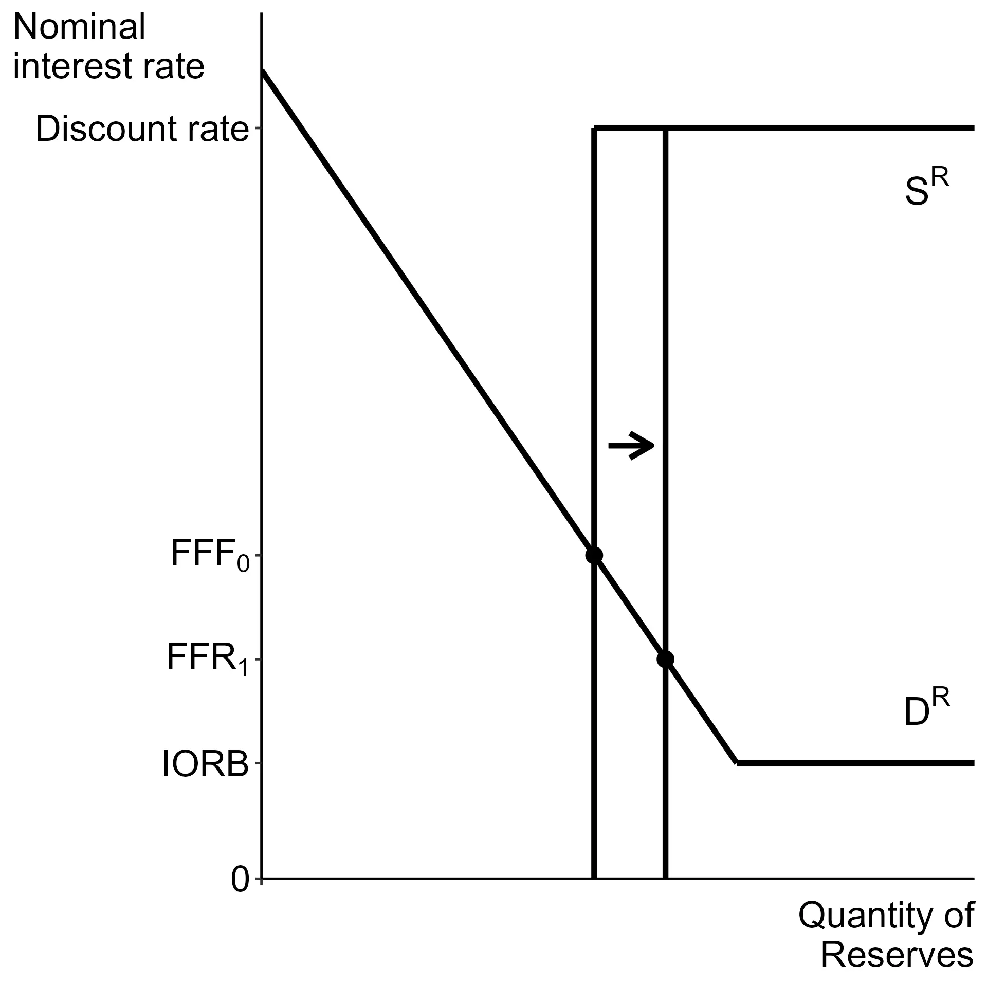
In an open market sale, the sold T-bills are bought by banks and other reserve market participants, which decreases the supply of reserves. Cash moves out of reserves in exchange for assets, so this action shifts the supply of reserves to the left and raises the equilibrium FFR.

An open market purchase reverses the story. Now the Fed buys T-bills in the reserves market. Banks gain reserves in exchange for assets. This increases the supply of reserves, shifting that curve to the right and lowering the equilibrium FFR.

Open market purchase increases reserves, leading to a cut in the federal funds rate.
Expansionary policy with limited reserves

As the amount of reserves changes, so does the amount of loans banks choose to make. These changes in loans then affect the money supply, as covered in the subchapter “Money supply expansion.” The exact impact on the money supply depends on the reserve ratio, desire of bank customers to hold currency, and the willingness of banks to hold excess reserves. We need to understand those links as concepts, but are not concerned with them in this market at this level.

Reserve ratio

As discussed in the previous subchapter, the reserve ratio is a shifter for the demand curve. An increase in the reserve ratio shifts DR​ to the left. It also lowers the money multiplier, which is the more important effect.

In the United States the reserve ratio was lowered to zero in March of 2020 and has remained there since. While it is good to understand how raising it would impact the reserves market, it is not currently relevant.

Discount rate

Recall that the discount rate determines the upper bound for the demand curve for reserves. In the limited reserves case changing the discount rate will not have an impact unless it is reduced below the current FFR rate. This may be relevant to the experience of some countries, but not for our usual central bank examples.

Monetary policy with ample reserves

The limited reserves case covered an equilibrium on the downward sloping portion of DR​. Now we will discuss the ample reserves case, where the equilibrium is on the flat portion of DR​. In this case the federal funds rate (FFR) is equal to the interest rate on reserve balances (IORB). In reality, they are not exactly equal, but we may discuss it as if they are.

With ample reserves the main tool from the limited reserves case, open market operations, should not impact the FFR. So the Fed needs alternate policy tools to impact interest rates and change the money supply.

Administrative rates

The discount rate, IOR and ON RRP rates are collectively called administrative rates. Recall that for the supply curve for reserves the discount rate provides the upper bound, while the interest rate on reserve balances and the overnight reverse repurchase rates provide the lower bound of demand for reserves. These can be changed together to change the upper and lower limits for the equilibrium interest rate, the FFR. Importantly, this is not a complete shift of either supply or demand.

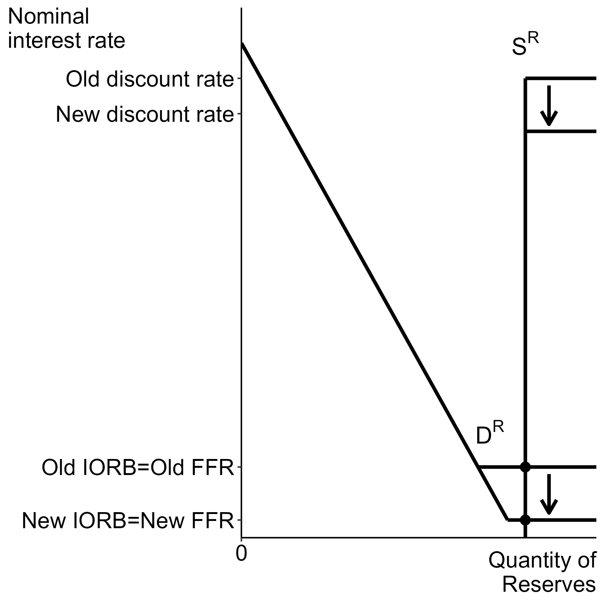
For example, to pursue expansionary policy and expand the money supply, the Fed needs to lower the FFR. To do this they lower all three administrative rates, which moves down both the upper and lower bound. Because SR​ crosses DR​ at the lower bound in the ample reserves case, lowering all three rates lowers the FFR.

A cut in both administrative rates leads to a cut in the federal funds rate.
Expansionary policy with ample reserves

To increase the FFR instead, the above story would simply take place in reverse. Raising all three administrative rates shifts the two horizontal portions up, leading to a higher equilibrium FFR.

Quantitative easing (QE)

The second alternate tool is quantitative easing. Quantitative easing refers to any time a central bank buys any assets not involved in open market operations, similar to open market purchases. Quantitative tightening (QT) is the term for the QE version of open market sales. This is the central bank selling assets purchased in previous rounds of QE.

Just like open market operations in the limited reserves case, QE can be thought of as shifting SR​ to the right. Regardless of the impact on reserves, QE always expands access to liquidity for banks and financial institutions.

However QE is mainly used in two situations, when interest rates are near zero and during a financial crisis. When interest rates are near zero standard monetary policy options cannot be used, a situation known as a liquidity trap. In a financial crisis changes in risk may remove the desire of banks to lend, lowering the money multiplier to near zero.

In each case, QE provides reserves to banks outside of the standard reserve market process. Thus QE enables banks to strengthen their balance sheets and at least theoretically should slightly increase lending.

In reality, it is not clear exactly how “successful” QE is as a policy. The link between reserve expansion under this policy and changes in the money supply is weaker than with open market operations in the limited reserves case. QE may push interest rates lower, but this can lead to banks taking on additional risk and cause different problems down the road.

The biggest problem is that the trade-offs undertaken with QE are more long term and thus are difficult to evaluate. The QE pursued during the Great Recession likely prevented additional failures of banks and financial firms. However, as of mid-2026 some of those assets purchased are still held by the Fed. QT was started in 2018 and paused in 2019, only for more QE to take place in 2020.

Limited reserves

  • Supply of reserves intersects demand on downward sloping portion
  • Open market operations (OMO) are primary Fed tool
    • Open market sale: Fed sells T-bills, decreases reserves, raises FFR (contractionary)
    • Open market purchase: Fed buys T-bills, increases reserves, lowers FFR (expansionary)
  • Changes in reserves affect loans and money supply
    • Impact depends on reserve ratio, currency demand, excess reserves

Reserve ratio

  • Reserve ratio shifts demand for reserves (DR​)
    • Increase shifts DR​ left
  • U.S. reserve ratio set to zero since March 2020

Discount rate (limited reserves)

  • Sets upper bound for demand curve
  • Changing discount rate only matters if below current FFR

Monetary policy with ample reserves

  • Equilibrium on inelastic (lower bound) portion of DR​
  • OMO does not impact FFR; alternate tools needed

Administrative rates

  • Discount rate, Interest on Reserves (IOR), Overnight Reverse Repurchase (ON RRP)
    • Set upper and lower bounds for DR​
  • Lowering all three rates lowers FFR (expansionary)
  • Raising all three rates increases FFR (contractionary)
  • Adjusting rates changes bounds, not whole curve

Quantitative easing (QE)

  • Central bank buys assets beyond standard OMO
    • Shifts SR​ right, but does not change FFR with ample reserves
  • Expands liquidity, may not increase lending/money supply
    • Banks may hold reserves for interest or balance sheet improvement
  • Used when OMO ineffective (e.g., liquidity trap, near-zero rates)
  • Quantitative tightening (QT): selling assets to unwind QE
  • QE examples: Fed purchases of MBS, long-term Treasuries (QE1, QE2, QE3)
  • Effects of QE less direct than OMO; long-term trade-offs, unclear effectiveness
Previous
Next  | 5.1 The Phillips curve
All rights reserved ©2016 - 2026 Achievable, Inc.

Implementation of monetary policy

In our market for reserves there was no specific restriction on where the supply for reserves intersects with the demand for reserves. We will now discuss the two most practical cases.

Limited reserves

The limited reserves case refers to the supply of reserves intersecting the demand for reserves on the downward sloping portion of the demand curve.

The limited reserves case provides a reliable overview of monetary policy operations before the Great Recession (pre-2008). In older AP Macroeconomics materials, this is the exclusive focus of discussions of monetary policy.

Open market operations

With limited reserves, shifting the supply curve of reserves causes changes to the federal funds rate directly. In a limited reserves world, open market operations are the primary tool of the Fed. The Fed sells T-bills in an open market sale and buys them in an open market purchase. Recall that T-bills are exclusively government bonds with a duration under 1 year (short term).

In an open market sale, the sold T-bills are bought by banks and other reserve market participants, which decreases the supply of reserves. Cash moves out of reserves in exchange for assets, so this action shifts the supply of reserves to the left and raises the equilibrium FFR.

An open market purchase reverses the story. Now the Fed buys T-bills in the reserves market. Banks gain reserves in exchange for assets. This increases the supply of reserves, shifting that curve to the right and lowering the equilibrium FFR.

As the amount of reserves changes, so does the amount of loans banks choose to make. These changes in loans then affect the money supply, as covered in the subchapter “Money supply expansion.” The exact impact on the money supply depends on the reserve ratio, desire of bank customers to hold currency, and the willingness of banks to hold excess reserves. We need to understand those links as concepts, but are not concerned with them in this market at this level.

Reserve ratio

As discussed in the previous subchapter, the reserve ratio is a shifter for the demand curve. An increase in the reserve ratio shifts DR​ to the left. It also lowers the money multiplier, which is the more important effect.

In the United States the reserve ratio was lowered to zero in March of 2020 and has remained there since. While it is good to understand how raising it would impact the reserves market, it is not currently relevant.

Discount rate

Recall that the discount rate determines the upper bound for the demand curve for reserves. In the limited reserves case changing the discount rate will not have an impact unless it is reduced below the current FFR rate. This may be relevant to the experience of some countries, but not for our usual central bank examples.

Monetary policy with ample reserves

The limited reserves case covered an equilibrium on the downward sloping portion of DR​. Now we will discuss the ample reserves case, where the equilibrium is on the flat portion of DR​. In this case the federal funds rate (FFR) is equal to the interest rate on reserve balances (IORB). In reality, they are not exactly equal, but we may discuss it as if they are.

With ample reserves the main tool from the limited reserves case, open market operations, should not impact the FFR. So the Fed needs alternate policy tools to impact interest rates and change the money supply.

Administrative rates

The discount rate, IOR and ON RRP rates are collectively called administrative rates. Recall that for the supply curve for reserves the discount rate provides the upper bound, while the interest rate on reserve balances and the overnight reverse repurchase rates provide the lower bound of demand for reserves. These can be changed together to change the upper and lower limits for the equilibrium interest rate, the FFR. Importantly, this is not a complete shift of either supply or demand.

For example, to pursue expansionary policy and expand the money supply, the Fed needs to lower the FFR. To do this they lower all three administrative rates, which moves down both the upper and lower bound. Because SR​ crosses DR​ at the lower bound in the ample reserves case, lowering all three rates lowers the FFR.

To increase the FFR instead, the above story would simply take place in reverse. Raising all three administrative rates shifts the two horizontal portions up, leading to a higher equilibrium FFR.

Quantitative easing (QE)

The second alternate tool is quantitative easing. Quantitative easing refers to any time a central bank buys any assets not involved in open market operations, similar to open market purchases. Quantitative tightening (QT) is the term for the QE version of open market sales. This is the central bank selling assets purchased in previous rounds of QE.

Just like open market operations in the limited reserves case, QE can be thought of as shifting SR​ to the right. Regardless of the impact on reserves, QE always expands access to liquidity for banks and financial institutions.

However QE is mainly used in two situations, when interest rates are near zero and during a financial crisis. When interest rates are near zero standard monetary policy options cannot be used, a situation known as a liquidity trap. In a financial crisis changes in risk may remove the desire of banks to lend, lowering the money multiplier to near zero.

In each case, QE provides reserves to banks outside of the standard reserve market process. Thus QE enables banks to strengthen their balance sheets and at least theoretically should slightly increase lending.

In reality, it is not clear exactly how “successful” QE is as a policy. The link between reserve expansion under this policy and changes in the money supply is weaker than with open market operations in the limited reserves case. QE may push interest rates lower, but this can lead to banks taking on additional risk and cause different problems down the road.

The biggest problem is that the trade-offs undertaken with QE are more long term and thus are difficult to evaluate. The QE pursued during the Great Recession likely prevented additional failures of banks and financial firms. However, as of mid-2026 some of those assets purchased are still held by the Fed. QT was started in 2018 and paused in 2019, only for more QE to take place in 2020.

Key points

Limited reserves

  • Supply of reserves intersects demand on downward sloping portion
  • Open market operations (OMO) are primary Fed tool
    • Open market sale: Fed sells T-bills, decreases reserves, raises FFR (contractionary)
    • Open market purchase: Fed buys T-bills, increases reserves, lowers FFR (expansionary)
  • Changes in reserves affect loans and money supply
    • Impact depends on reserve ratio, currency demand, excess reserves

Reserve ratio

  • Reserve ratio shifts demand for reserves (DR​)
    • Increase shifts DR​ left
  • U.S. reserve ratio set to zero since March 2020

Discount rate (limited reserves)

  • Sets upper bound for demand curve
  • Changing discount rate only matters if below current FFR

Monetary policy with ample reserves

  • Equilibrium on inelastic (lower bound) portion of DR​
  • OMO does not impact FFR; alternate tools needed

Administrative rates

  • Discount rate, Interest on Reserves (IOR), Overnight Reverse Repurchase (ON RRP)
    • Set upper and lower bounds for DR​
  • Lowering all three rates lowers FFR (expansionary)
  • Raising all three rates increases FFR (contractionary)
  • Adjusting rates changes bounds, not whole curve

Quantitative easing (QE)

  • Central bank buys assets beyond standard OMO
    • Shifts SR​ right, but does not change FFR with ample reserves
  • Expands liquidity, may not increase lending/money supply
    • Banks may hold reserves for interest or balance sheet improvement
  • Used when OMO ineffective (e.g., liquidity trap, near-zero rates)
  • Quantitative tightening (QT): selling assets to unwind QE
  • QE examples: Fed purchases of MBS, long-term Treasuries (QE1, QE2, QE3)
  • Effects of QE less direct than OMO; long-term trade-offs, unclear effectiveness

More from Financial sector

  • Closed economy loanable funds market
  • Macroeconomic finance
  • Financial assets and markets
  • Introduction to money
  • Simple money market