




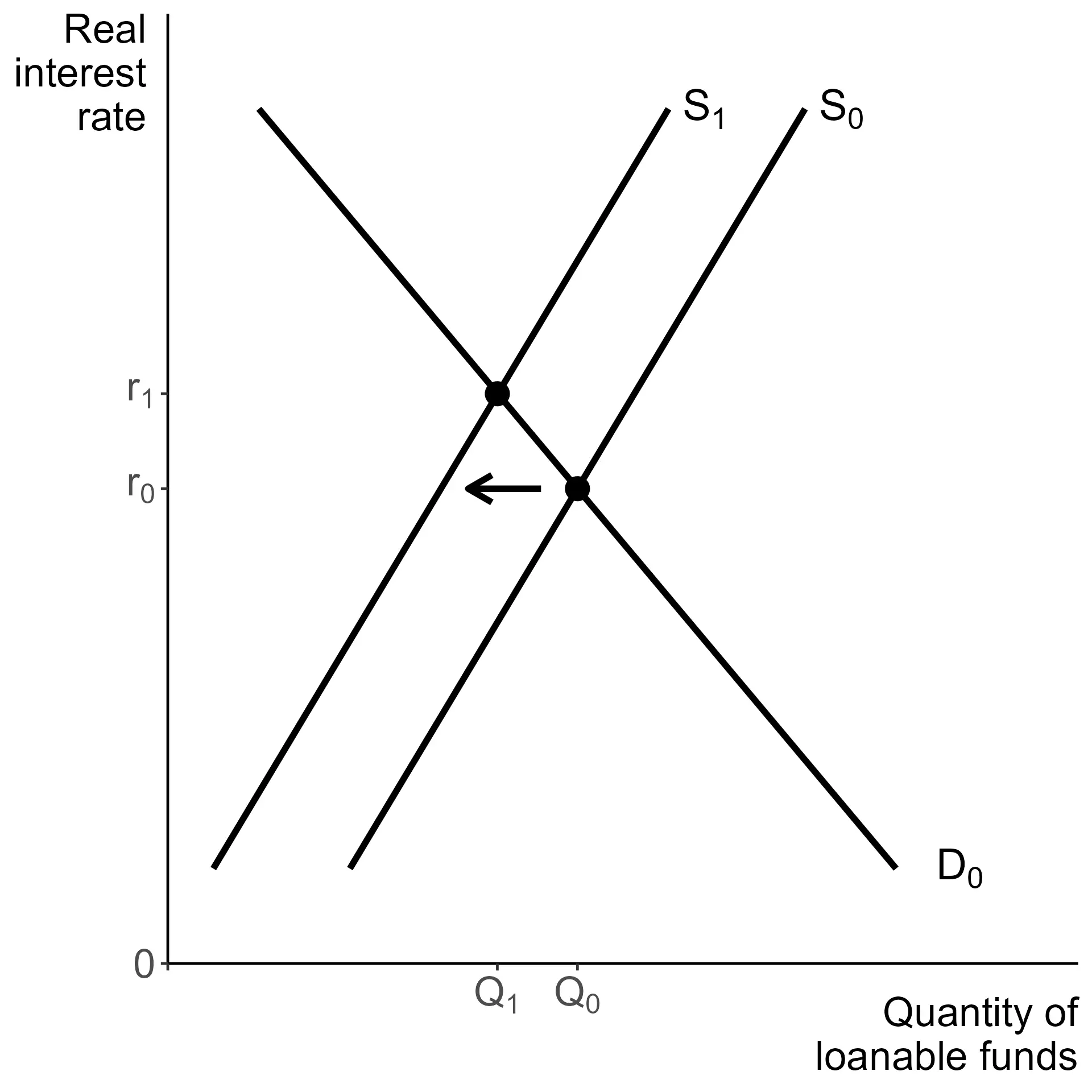
Closed economy loanable funds market
Our discussion of the financial sector begins with the loanable funds market in a closed economy. So there is no trade or international financial flows, which will be added in a future chapter.
We have seen savings and investment in our GDP accounting, and they must be exactly equal in a closed economy. The loanable funds market will provide more context into how the interest rate interacts with each of these individually and how it forces them to be equal.
The loanable funds market has the interest rate on the y-axis and the quantity of funds on the x-axis. We imagine lending and borrowing as a unified market with a single interest rate that is the same for borrowers and sellers. This interest rate should be thought of as the long-term interest rate. The market that determines the short-term rate will be discussed later.
While this is not completely realistic, adding real life details does not significantly change our main results.
Supply
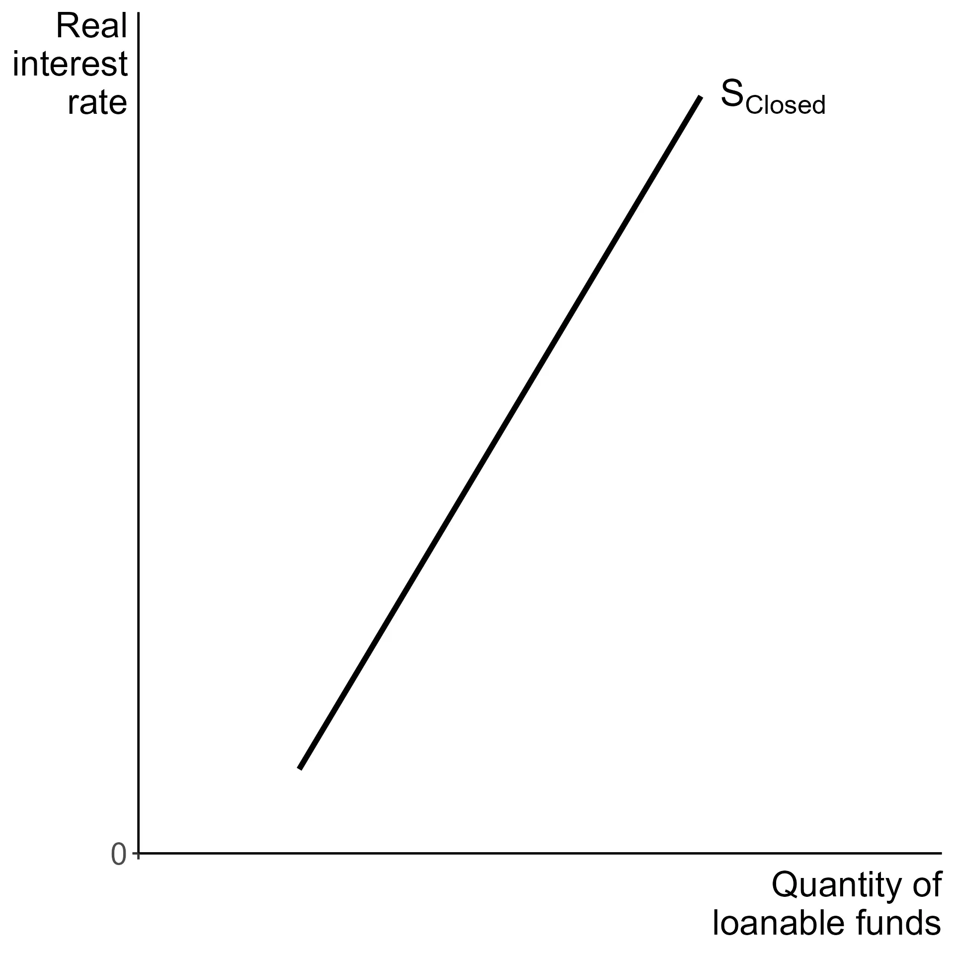
In a closed economy the supply of loanable funds comes exclusively from total savings. A normal supply curve comes from firms, but the supply for loanable funds comes from households. At the macro level this includes all funds not used for current period consumption. To name a few examples, contributions to retirement accounts, money put into investments, money put in a savings account, or even just money left in a checking account that is not spent by the end of the year.
An increase in the interest rate increases the opportunity cost of spending money today, and in response households will shift some consumption to savings. Thus all else equal, when the interest rate rise the amount of savings rises. From this we get our usual upward sloping supply curve.
The other source of loanable funds is the government. If the government has a surplus, that would add to supply. If the government runs a deficit, that would lower the supply. This amount does not depend on interest rates, it is chosen by government policy.
Shifters
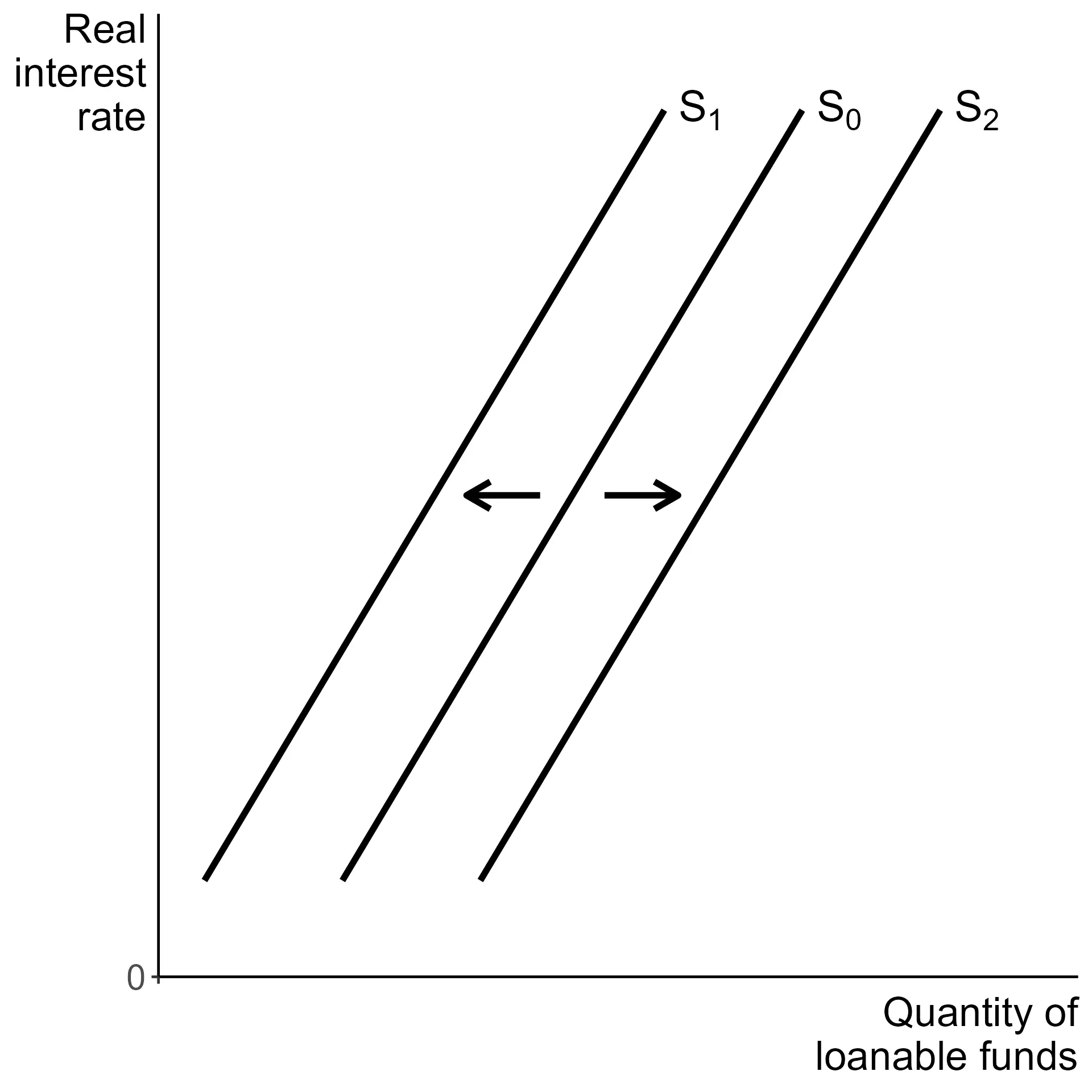
The shifters of supply will mostly be a variety of factors other than interest rates, which change the desire of households to save. The remaining factors all have to do with changes in the government budget situation.
Because the supply of loanable funds comes from households, many of the shifters are demand shifters for consumption. However for loanable funds, these shift the supply curve in the opposite direction as any shift in consumption. This reflects the tug-of-war between consumption and savings for a fixed level of income.
| Shifter | (left) | (right) |
|---|---|---|
| Inflation expectations | Lower | Higher |
| Future economic uncertainty | Higher | Lower |
| Household wealth | Decrease | Increase |
| Desire to consume () | Decrease | Increase |
| Household income | Increase | Decrease |
| Desire to save () | Increase | Decrease |
| Government budget | Surplus | Deficit |
| Government budget | Less borrowing | More borrowing |
Higher expectations of inflation reduce the real value of savings, and thus shift the supply of savings to the left. Higher uncertainty about the future, for example increased fear of a coming recession, lead households to save more and thus shifts the supply of savings to the right. This is called precautionary savings. Precautionary motives will be critical once we stop assuming all investments are identical.
Household wealth can often be thought of as being closely tied to the stock market or housing market. Higher wealth is generally thought to lead to lower saving or even borrowing on a micro level, so it shifts the supply curve to the left. This is the same as an increase in the from the consumption function.
Higher income has the opposite effect, leading households to save more for each value of the real interest rate. A higher , an increased preference for savings, causes the same shift.
Each of these affect the size of our two multipliers. Both the spending and tax multipliers are larger when is higher or when is lower. This makes fiscal policy cause larger shifts in the curve.
If the government runs a deficit when it previously had a balanced budget or if it borrows more than it had previously, that shifts the savings curve left. Taking a balanced budget to a surplus or borrowing less shifts the savings curve to the right.
Because the supply curve is upward sloping, when describing the shift we can say it represents a lower willingness to save for every interest rate or that a higher interest rate is needed to maintain the same quantity of savings.
Demand
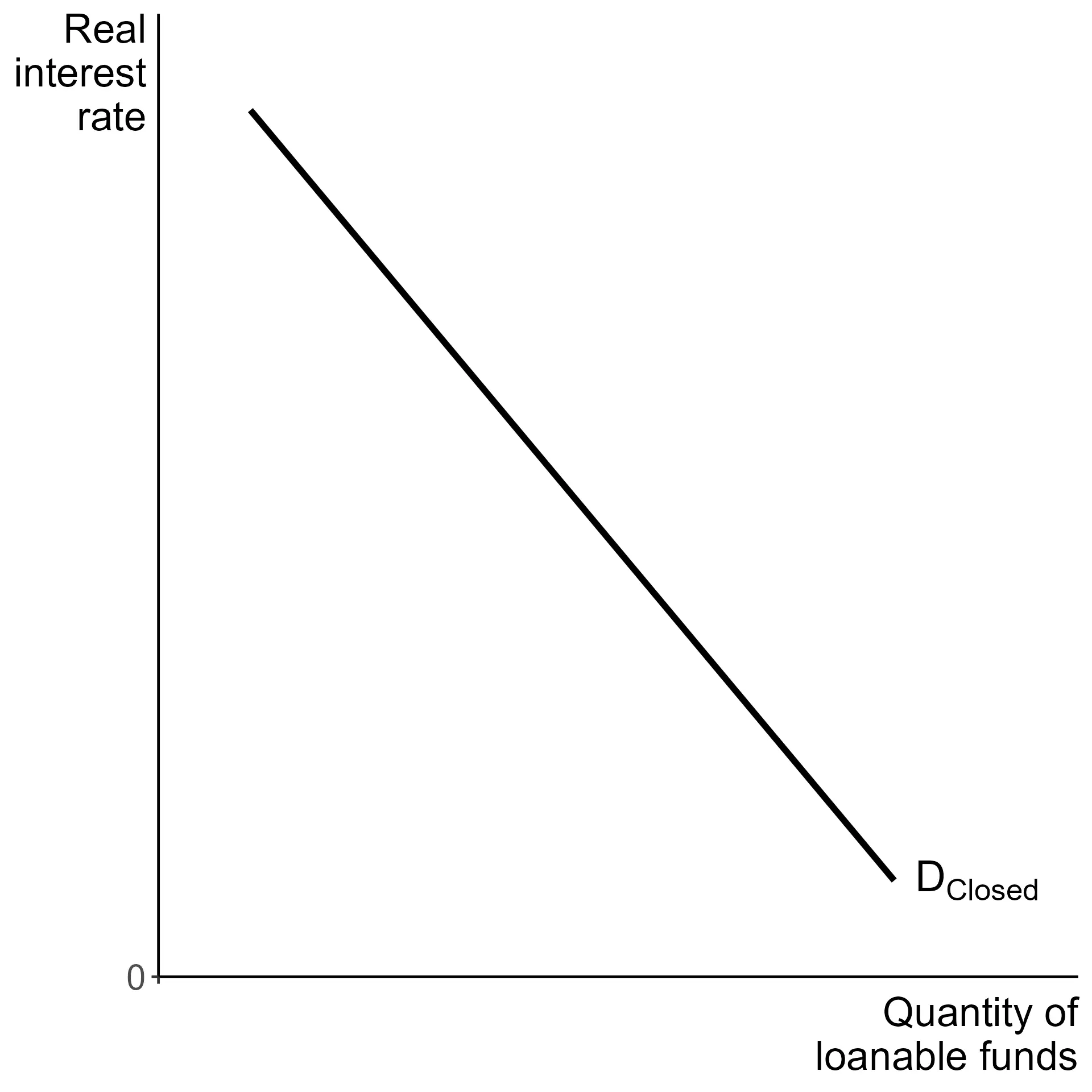
Just as with supply, the source of demand is flipped compared to our usual stories. For our purposes demand for loanable funds is the same as investment spending. In a closed economy it comes solely from private firms. This is downward sloping in the interest rate, at least partially because the interest rate represents the “price” of not investing. It is the opportunity cost of using funds for an investment, where the next best use of those funds is earning interest at the risk-free rate.
A second way to think of the inverse relationship between interest rates and demand for loanable funds is to consider what return a project needs to earn to be a worthwhile investment. It will be helpful to set aside uncertainty and speak as if project returns are guaranteed. We can imagine each firm has a schedule of potential investments, ordered from highest to lowest returns. For any interest rate, firms will pursue projects offering returns equal to or above that rate. Thus at worst any invested funds earn a rate equal to the risk-free option of an interest earning account.
No matter which explanation we rely on, as interest rates fall, a higher quantity of investments are worth pursuing.
Shifters
Because demand is sourced from firms, the shifters of demand in this market will be more closely aligned with the shifters of supply in other examples.
| Shifter | (more) | (less) |
|---|---|---|
| Business confidence | Increase | Decrease |
| “Animal spirits” | ||
| Subsidies for businesses subsidies | Increase | Decrease |
| Improvements in technology | Increase | Decrease |
| Expectations of future demand | Increase | Decrease |
| Taxes on businesses | Decrease | Increase |
| Risk or uncertainty | Decrease | Increase |
Anything that makes projects more profitable will increase demand for loanable funds and shift the curve to the right. General business sentiment is a key factor in movements in the stock market as a whole. This connects to what Keynes referred to as the “animal spirits,” with the bull referring to positive sentiment and bear referring to negative sentiment.
It can be helpful to relate other factors to the nebulous example of animal spirits. Bullish sentiment shifts the demand for loanable funds to the right. Reductions in taxes, increases in subsidies, improvements in technology, and expectations of higher prices or higher demand in the future all have similar effects.
Bearish factors include anything that makes projects less profitable. these decrease demand and cause a leftward shift. Examples of this include increases in uncertainty and risk, expectations of less desirable future business conditions (lower demand or lower prices).
For example, if there is a new expectation of lower market demand or lower prices in the future for any reason, a previously planned project to build a factory may be cancelled.
Equilibrium
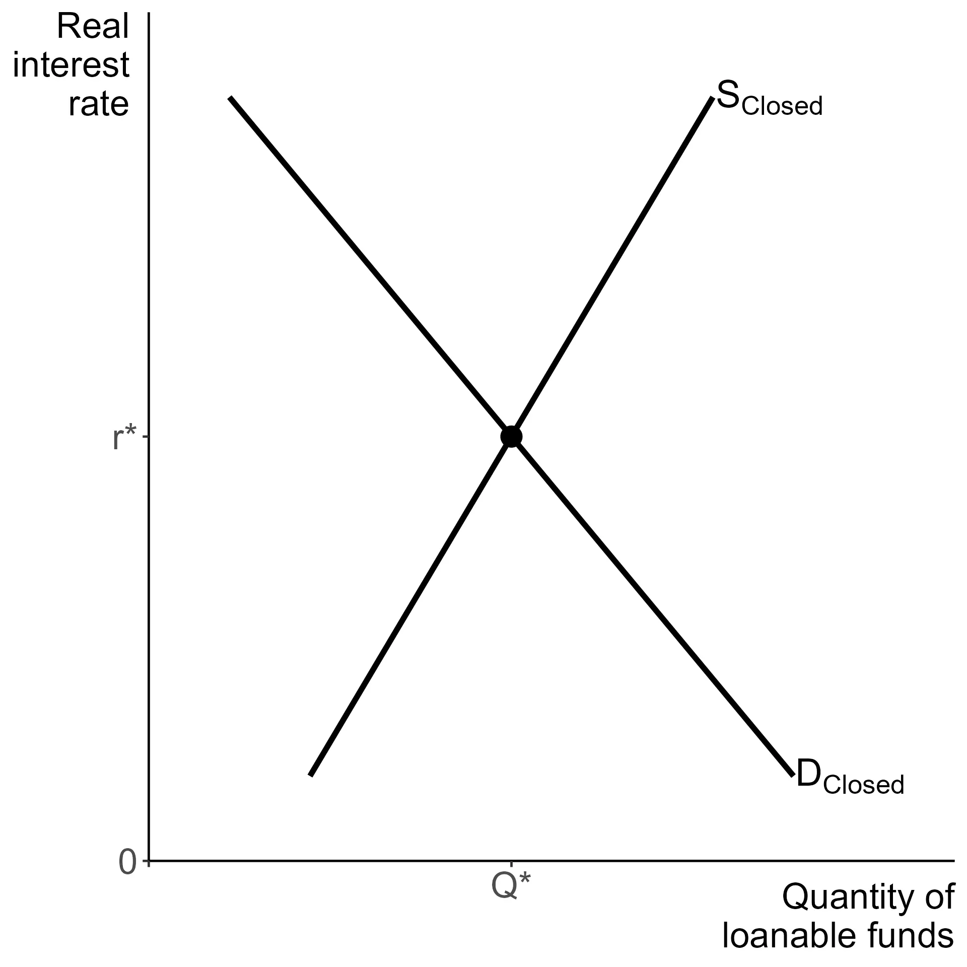
In the closed economy version of the loanable funds market, the equilibrium is set by the intersection of supply and demand and the equilibrium quantity of loanable funds is the same as the amount of investment.
Up to now we have not concerned ourselves with the practical details of how buyers and sellers meet. For the loanable funds market it is a complex process involving other economic actors.
A financial intermediary is any entity that connects savers and borrowers. They often have specialized roles that focus on a few key functions. Examples include banks, credit unions, investment brokers, pension funds and insurance companies. Besides linking borrowers and savers, they provide benefits such as risk management and risk sharing, and make it easier to convert investments into cash.
Shifters and equilibrium
Following our earlier examples, first consider a shift of to the left. Now at every interest rate the quantity supplied is lower, while there was no change to the quantity demanded. So there is a mismatch between supply and demand at the original equilibrium interest rate (), with a higher quantity demanded. To incentivize the addition of funds to this market, interest rates must rise. As that happens, there is both an increase in the quantity supplied and a decrease in the quantity demanded. This leads to a new equilibrium at and .
Finally, here we present again the table of the effects of various shifts on the market equilibrium, for the specific case of the loanable funds market.
| Shift or shifts | Change in | Change in |
|---|---|---|
| Higher | Lower | |
| Lower | Higher | |
| Lower | Higher | |
| Higher | Lower | |
| and | Unknown | Higher |
| and | Unknown | Lower |
| , | Lower | Unknown |
| , | Higher | Unknown |
Higher demand or lower supply lead to higher interest rates. Lower demand or higher supply lead to lower interest rates. All else equal, for a single shift quantity moves in the same direction as demand and in the opposite direction as supply.