


Achievable logoAchievable logo
AP Macroeconomics
Sign in
Sign up
Purchase
Textbook
Practice exams
Support
How it works
Exam catalog
Mountain with a flag at the peak
Textbook
Example
1. Core economic concepts
2. Measurement of economic performance
3. Modeling of income and prices
4. Financial sector
5. Long-run consequences of stabilization policy
5.1 The Phillips curve
5.2 Fiscal policy in the long run
5.3 Monetary policy in the long run
5.4 Stagflation
6. Open economy
Achievable logoAchievable logo
5.1 The Phillips curve
Achievable AP Macroeconomics
5. Long-run consequences of stabilization policy
Our AP Macroeconomics course is currently in development and is a work-in-progress.

The Phillips curve

7 min read
Font
Discuss
Share
Feedback

The Phillips curve is our final concept for the short run and our first concept for the long run. It has the inflation rate is on the y-axis and the unemployment rate is on the x-axis.

It can be helpful to view this as nothing more than a transformation of the AD-AS model, with a focus on the labor market directly instead of real GDP. Again we will see that in the short run there is a trade-off between prices and economic activity, while in the long run there is not.

Short run Phillips curve

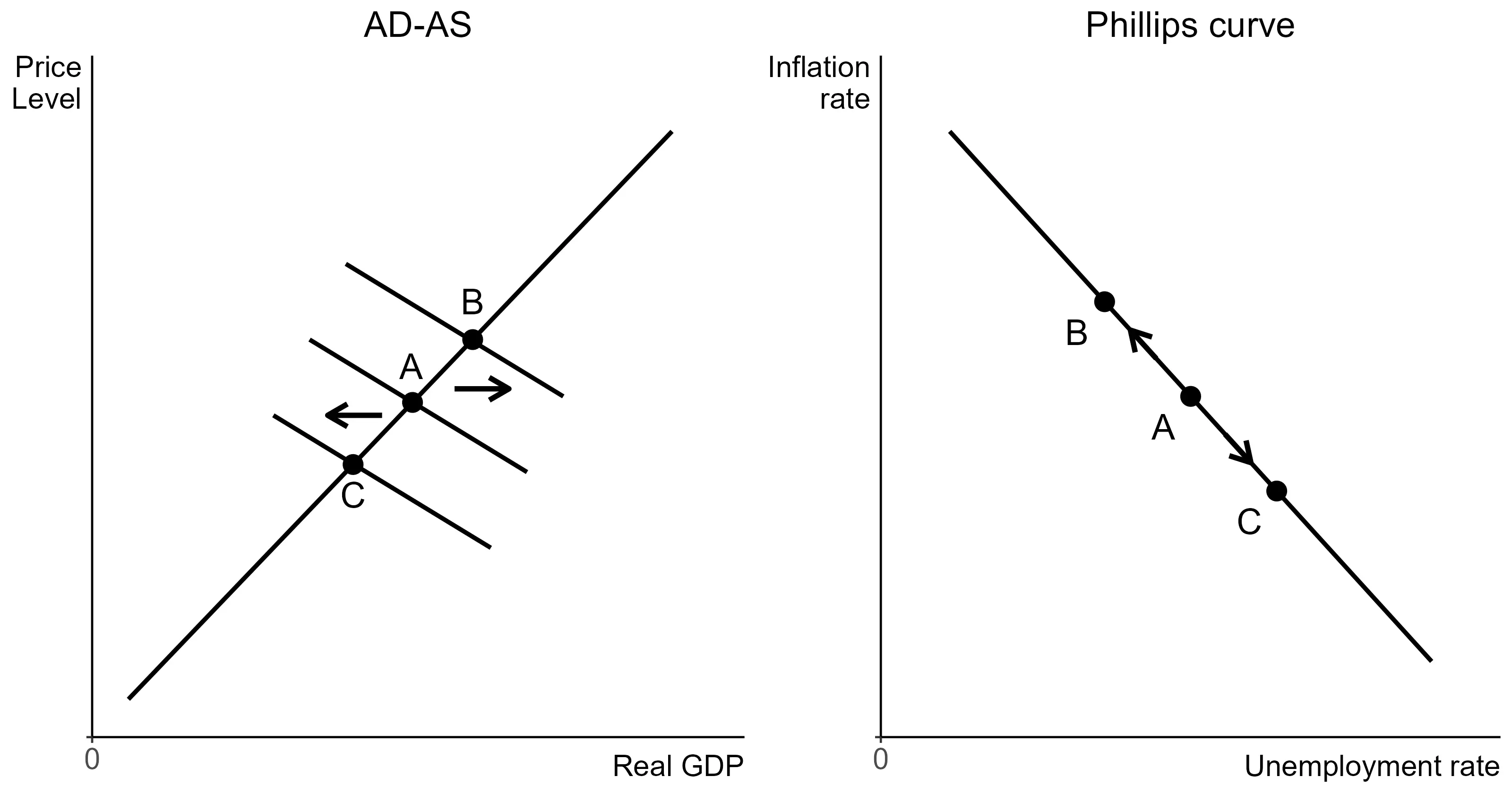
We begin with a short run equilibrium in the AD-AS model. From this, if AD shifts to the right, Y and PL both rise. Another way to view these changes is as an increase in inflation and a reduction in the unemployment rate, a movement from point A to point B in each graph.

Shifting the $AD$ curve as a movement along the short run Phillips curve.
AD-AS and the SRPC

If AD shifts left, the opposite occurs. PL is lower, which is the same as lowering inflation, and Y is lower, which is the same as raising the unemployment rate. This is a movement from point A to point C in each graph. Changes in the AD are always movements along a single short run Phillips curve.

One lesson from the short run AD-AS model was that there is a trade-off between the price level and production. What the SRPC does is highlight that there is also a tradeoff between inflation and unemployment in the short run. This trade-off exists for the same reason that SRAS is upward sloping, sticky prices.

Shifters

Because the SRPC mirrors the SRAS, one might guess that the shifters are the same and that is completely correct. Be careful that while the shifts are the same conceptually, they are in the opposite direction as SRAS shifts. For that reason, it can be slightly more intuitive for explanations to refer to shifts in the short run Phillips curve as up and down instead of left and right.

Shifter SRPC→ (up) SRPC← (down)
Supply shock Negative Positive
Expected inflation Higher Lower

Higher expected inflation or a negative supply shock leads to higher inflation for every level of unemployment (output). Either of these shift SRAS left and the SRPC up (right).

Lower expected inflation or a positive supply shock have the opposite effect. Lower inflation for every level of unemployment (output). So these shift SRAS right and the SRPC down (left).

The long run

Just as the short run Phillips curve is connected to short run aggregate supply, the long run Phillips curve is linked to long run aggregate supply.

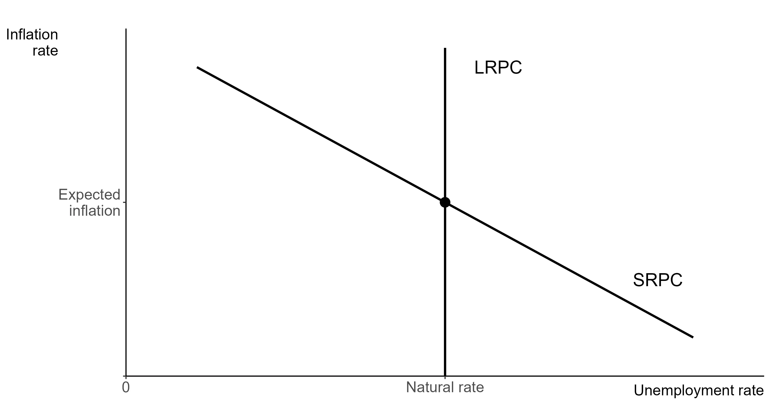
Just as with aggregate supply, the long run version is vertical. Recall that the LRAS curve is vertical at Y⋆, which is the level of output associated with the natural rate of unemployment, u⋆. The long run Phillips curve (LRPC) is vertical at u⋆.

Again the trade-off of the short run disappears in the long run. This is because in the long run wages fully adjust, so inflation must be equal to expected inflation and output must return to the full employment level.

Adding a vertical long run Phillips curve to the downward sloping short run Phillips curve.
Phillips curve in the long run and short run

The short run Phillips curve crosses the long run Phillips curve at the expected rate of inflation. This is what is different than the aggregate supply and aggregate demand model. There we had no specific price level where the short and long run curves crossed.

Shifters

Shifters of the LRPC are more limited than those of the LRAS curve. The only shifters are factors that change the natural rate of unemployment. So anything that adjusts the level of frictional or structural unemployment in the economy will also shift the long run Phillips curve.

Shifter LRPC→ LRPC←
Demographic changes Negative Positive
Labor market conditions Weaker Stronger

A demographic change may stem from differences in the size of generations, immigration, education and gender. An ongoing story is the retirement of the baby boomer generation. It is larger than the cohorts that follow, so as they begin to retire that will lead to the labor force shrinking. This may cause shortages of workers with education and training in specific sectors, such as healthcare or software engineering.

Globalization and expanded trade can also lead to shifts in the location of production, leaving unemployed workers who may have difficulty transitioning to the jobs that remain available.

Labor market conditions cover items mentioned earlier, for example laws regulating hours and working conditions. It also includes technological innovations. The advent of the internet and job websites could be thought to reduce frictional unemployment, making the process of changing jobs faster.

Transition from short run to long run

In the AD-AS model, prices adjust causing a shift in SRAS which returns output to potential GDP. In the Phillips curve, the adjustment comes from changes in expected inflation.

We mostly do not concern ourselves with how inflation expectations are formed. The sequence of events is what is likely to show up at least once on the test. In the Phillips curve story, expectations of inflation align with actual inflation and shift the short run curve to intersect the long run curve at that inflation rate. So all we assume is that in the long run inflation expectations match actual inflation.

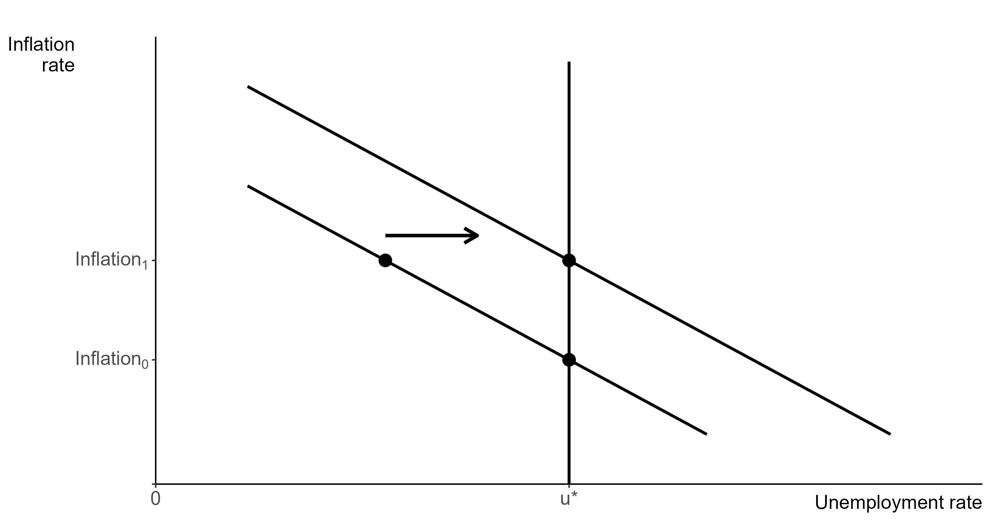
This is almost perfectly identical to the long run adjustment in the AD-AS model. There price adjustments shift the SRAS curve so that AD, LRAS and SRAS all cross at Y⋆. In the Phillips curve, if we are not in a long run equilibrium then expected inflation changes to match actual inflation and the SRPC shifts to cross the LRPC at the natural rate of unemployment.

Changing inflation expectations shifting the $SRPC$ so the equilibrium is actual inflation and the natural rate of unemployment.
Long run adjustment of the Phillips curve

The graph shows the example of an inflationary gap. This moves the economy up the SRPC, raising inflation to Inflation0​ and lowers unemployment. When expectations fully adjust to the new level of inflation, there is a shift to a new SRPC and the economy returns to full employment at u⋆.

Previous
Next  | 5.2 Fiscal policy in the long run
All rights reserved ©2016 - 2026 Achievable, Inc.

The Phillips curve

The Phillips curve is our final concept for the short run and our first concept for the long run. It has the inflation rate is on the y-axis and the unemployment rate is on the x-axis.

It can be helpful to view this as nothing more than a transformation of the AD-AS model, with a focus on the labor market directly instead of real GDP. Again we will see that in the short run there is a trade-off between prices and economic activity, while in the long run there is not.

Short run Phillips curve

We begin with a short run equilibrium in the AD-AS model. From this, if AD shifts to the right, Y and PL both rise. Another way to view these changes is as an increase in inflation and a reduction in the unemployment rate, a movement from point A to point B in each graph.

If AD shifts left, the opposite occurs. PL is lower, which is the same as lowering inflation, and Y is lower, which is the same as raising the unemployment rate. This is a movement from point A to point C in each graph. Changes in the AD are always movements along a single short run Phillips curve.

One lesson from the short run AD-AS model was that there is a trade-off between the price level and production. What the SRPC does is highlight that there is also a tradeoff between inflation and unemployment in the short run. This trade-off exists for the same reason that SRAS is upward sloping, sticky prices.

Shifters

Because the SRPC mirrors the SRAS, one might guess that the shifters are the same and that is completely correct. Be careful that while the shifts are the same conceptually, they are in the opposite direction as SRAS shifts. For that reason, it can be slightly more intuitive for explanations to refer to shifts in the short run Phillips curve as up and down instead of left and right.

Shifter SRPC→ (up) SRPC← (down)
Supply shock Negative Positive
Expected inflation Higher Lower

Higher expected inflation or a negative supply shock leads to higher inflation for every level of unemployment (output). Either of these shift SRAS left and the SRPC up (right).

Lower expected inflation or a positive supply shock have the opposite effect. Lower inflation for every level of unemployment (output). So these shift SRAS right and the SRPC down (left).

The long run

Just as the short run Phillips curve is connected to short run aggregate supply, the long run Phillips curve is linked to long run aggregate supply.

Just as with aggregate supply, the long run version is vertical. Recall that the LRAS curve is vertical at Y⋆, which is the level of output associated with the natural rate of unemployment, u⋆. The long run Phillips curve (LRPC) is vertical at u⋆.

Again the trade-off of the short run disappears in the long run. This is because in the long run wages fully adjust, so inflation must be equal to expected inflation and output must return to the full employment level.

The short run Phillips curve crosses the long run Phillips curve at the expected rate of inflation. This is what is different than the aggregate supply and aggregate demand model. There we had no specific price level where the short and long run curves crossed.

Shifters

Shifters of the LRPC are more limited than those of the LRAS curve. The only shifters are factors that change the natural rate of unemployment. So anything that adjusts the level of frictional or structural unemployment in the economy will also shift the long run Phillips curve.

Shifter LRPC→ LRPC←
Demographic changes Negative Positive
Labor market conditions Weaker Stronger

A demographic change may stem from differences in the size of generations, immigration, education and gender. An ongoing story is the retirement of the baby boomer generation. It is larger than the cohorts that follow, so as they begin to retire that will lead to the labor force shrinking. This may cause shortages of workers with education and training in specific sectors, such as healthcare or software engineering.

Globalization and expanded trade can also lead to shifts in the location of production, leaving unemployed workers who may have difficulty transitioning to the jobs that remain available.

Labor market conditions cover items mentioned earlier, for example laws regulating hours and working conditions. It also includes technological innovations. The advent of the internet and job websites could be thought to reduce frictional unemployment, making the process of changing jobs faster.

Transition from short run to long run

In the AD-AS model, prices adjust causing a shift in SRAS which returns output to potential GDP. In the Phillips curve, the adjustment comes from changes in expected inflation.

We mostly do not concern ourselves with how inflation expectations are formed. The sequence of events is what is likely to show up at least once on the test. In the Phillips curve story, expectations of inflation align with actual inflation and shift the short run curve to intersect the long run curve at that inflation rate. So all we assume is that in the long run inflation expectations match actual inflation.

This is almost perfectly identical to the long run adjustment in the AD-AS model. There price adjustments shift the SRAS curve so that AD, LRAS and SRAS all cross at Y⋆. In the Phillips curve, if we are not in a long run equilibrium then expected inflation changes to match actual inflation and the SRPC shifts to cross the LRPC at the natural rate of unemployment.

The graph shows the example of an inflationary gap. This moves the economy up the SRPC, raising inflation to Inflation0​ and lowers unemployment. When expectations fully adjust to the new level of inflation, there is a shift to a new SRPC and the economy returns to full employment at u⋆.

More from Long-run consequences of stabilization policy

  • Fiscal policy in the long run
  • Monetary policy in the long run
  • Stagflation