Monetary policy in the long run | AP Macro Long-run consequences of stabilization policy

In the short run, monetary policy stimulates the economy as fiscal policy does although exactly how this occurs is not the same. Monetary policy changes interest rates, which affects the money supply. This shifts $A D$ , to the right if interest rates are lower (higher money supply) and to the left if interest rates are higher (lower money supply).

In the long run, the self-adjustment mechanism of all wages and prices fully adjusting always brings the economy back to full employment. So the economy returns to the initial level of GDP and unemployment for any shift in $A D$ or any temporary supply shock to $SR A S$ . Because monetary policy is one of those $A D$ shifters, we end up with our long run result rather efficiently.

Definitions

Neutrality of money: In the long run, changes in the money supply affect the price level but do not affect real output.

This is a direct outcome of a vertical $L R A S$ and $L RPC$ , due to prices fully adjusting and matching expectations in the long run. Money can affect nominal variables, but not real ones.

Put another way, monetary factors are not shifters of either curve. Thus monetary policy can be used to counter a recession and possibly a supply shock or stagflation, but it cannot be used to generate long run growth.

Monetary overshooting

Recognition and decision lags can be relatively fast for monetary policy. FOMC meetings can be held outside of the regular schedule in order to respond more quickly to a crisis.

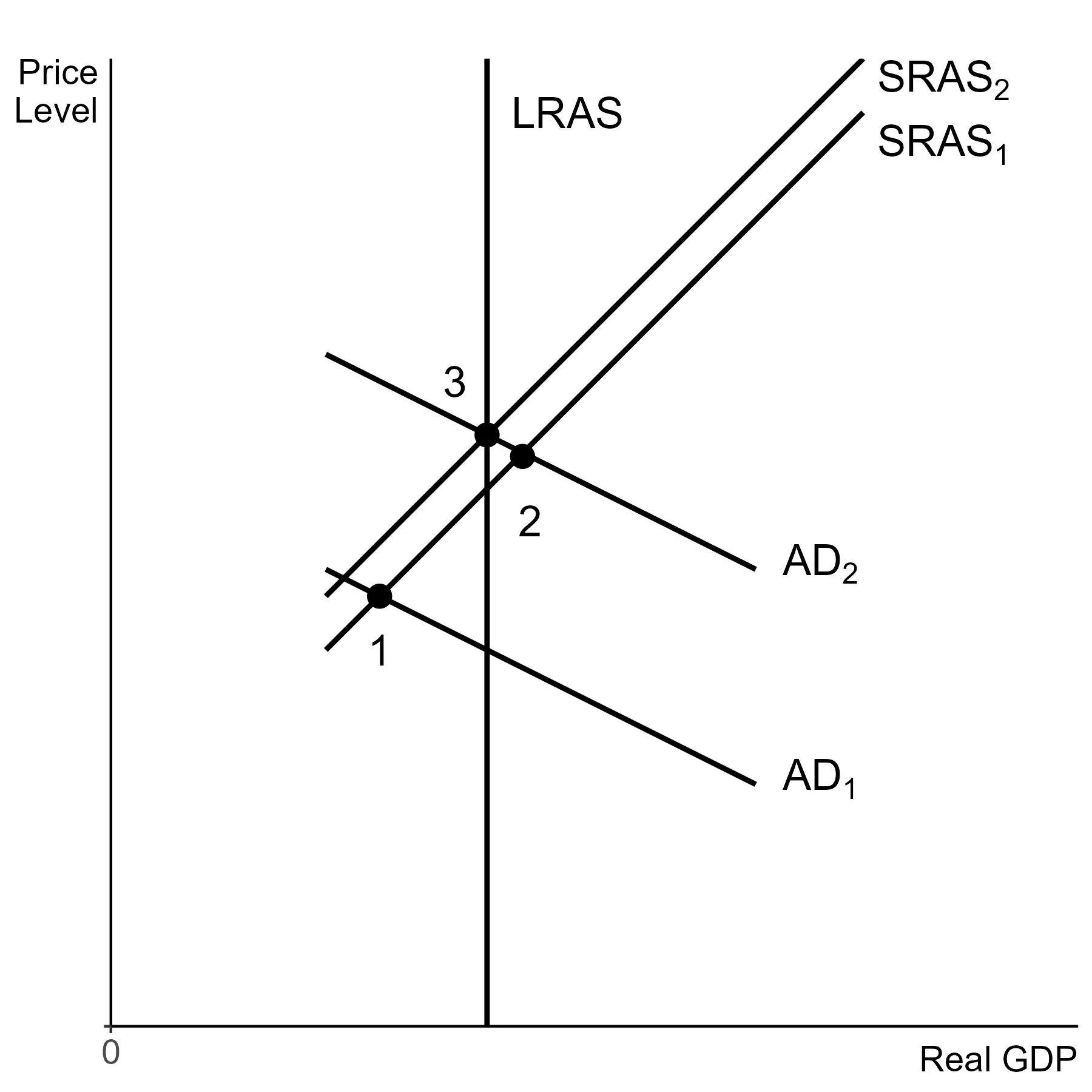
However, implementation lag is slower than fiscal policy. This means that monetary policy will overshoot, or push the economy past full employment in the short run. In the chart below, this is represented by a movement from point $1$ to point $2$ .

$AD$ shifts past $LRAS$ due to monetary policy, so the transition to long run leads to even higher inflation. — Monetary policy overshooting

The long run adjustment from point $2$ is no different than any other. Inflation expectations will rise, leading $SR A S$ to shift left and to an increase in the price level. The economy settles into a new long run equilibrium at point $3$ . Monetary policy does close the recessionary gap in the long run, but can be considered to cause additional inflation due to implementation lag.

Money is neutral but monetary policy by itself can be expected to cause small amounts of extra inflation.

The long run neutrality of money is reinforced by a final important concept connecting the money supply to spending in the economy.

Quantity theory of money

The impact of money supply changes on the price level can even be measured in a relatively straightforward way. That requires an equation known as the quantity theory of money.

$M \times V = P \times Y$

Three of the pieces of this equation are things we have seen before:

M = money supply
P = price level (for example the GDP deflator)
Y = real GDP

And one we have not seen before:

V = velocity of money

The velocity of money is the average number of times a dollar is spent in a year. For our purposes, we can treat velocity as stable. If it is not constant, it is close enough to constant in the long run.

The left side of this equation is $M \times V$ , which is total spending in the entire economy in a year. The right hand side is $P \times Y$ , which is the value of all goods purchased in the economy in a given year. In other words, nominal GDP. So the quantity theory says that the flow of dollars in the economy must enable the purchase of all goods that were produced.

Velocity being constant means that if the money supply grows faster than real output then the price level must rise. So not only does money not affect real production in the long run, the only long run outcome of increasing the money supply is inflation.

For AP Macroeconomics, this is a conceptual framework and an identity. You will not have to re-arrange this, only complete relatively simple calculations. You may be expected to use the fact that if velocity is constant,

$Inflation = Money supply growth - Real GDP growth .$

To make it as clear as possible, here’s a quick example of the highest math difficulty to expect.

Q: If the money supply increases by 5%, and real GDP is the same as last year. What does the quantity theory of money predict inflation will be?

The same as the previous year
0%
5%
3%
-5%

Answer below.

(spoiler)

5%, What the quantity theory tells us is that money supply growth beyond the rate of GDP growth must lead to inflation. So with constant real GDP, inflation is the same as the growth rate of money.

Finally, this result of the quantity theory makes it clear what we would expect as a side-effect of printing money to pay for government budget deficits rather that using tax revenue. Printing money that is not a response to real GDP growth only leads to inflation.

Completing a back of the envelope calculation for the US in 2025, government spending was roughly 25% of M2 and real GDP growth was just short of 2%. So if the government raised no tax revenue at all and only printed money to fund current expenditures, the quantity theory suggests that would cause 25%-2%=23% inflation.

Printing money to pay for government budget deficits are often a significant contributor to, if not the main cause of, historical episodes of hyperinflation. Inflation expectations rise and prices rise, so the government has to print even more money to make purchases or fund desired programs. So inflation expectations and prices continue to rise, and things can quickly get out of control.

That being said, the quantity theory is a long run relationship. If the government started printing money to pay for its spending, it would occur in smaller pieces throughout the year.