What you’ll learn:

• How to approximate the area under a curve using rectangles (Riemann sums) and trapezoids
• Calculate Riemann sums for intervals of unequal widths
• Interpret whether left or right sums over- or underestimate based on the function’s behavior

In the previous section, areas were easy to find because the regions were simple geometric shapes. Now suppose you want the area under a curved graph, like $f(x)=x^2$, from $x=a$ to $x=b$. Before learning how to find the exact area, it helps to start with an approximation.

A common approach is to break the interval into smaller pieces, approximate the region with rectangles (or trapezoids), and add up their areas. This idea leads to Riemann sum approximations.

Riemann sums to estimate area

There are 3 main types of Riemann approximations: left, right, and midpoint Riemann sums. All three use rectangles.

Another common approximation is the Trapezoidal rule, which uses trapezoids. It isn’t technically a Riemann sum, but it follows the same “partition and add” process.

Here are the steps to finding a Riemann sum:

1. Divide the interval $[a,b]$ into $n$ subintervals, where each subinterval has equal width $\Delta x$:

$$\Delta x=\frac{b-a}{n}$$

2. On each subinterval, choose a point $x_k$ to evaluate the function (this choice depends on which type of Riemann sum you’re using).

3. Multiply the function value $f(x_k)$ by the width $\Delta x$to get the area of a rectangle.
   For a trapezoid,$\Delta x$ is the height of each trapezoid while the function values are the bases.

   • Note: If the function value is negative, the rectangle lies below the $x$-axis, so its contribution is negative. That’s expected here because we’re approximating net signed area, which accounts for both positive and negative values.

4. Add the areas together.

Examples

Estimate the area under $f(x)=x^2$ with $n=4$ subintervals on the interval $[1,5]$using a:

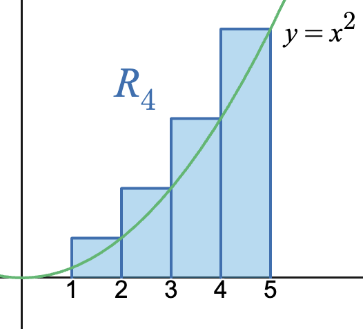
a) Right Riemann sum
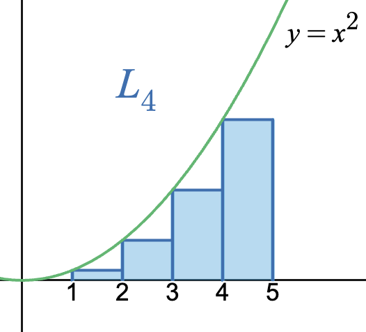
b) Left Riemann sum
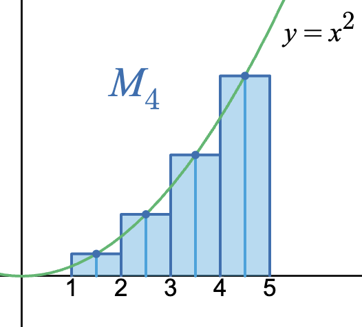
c) Midpoint Riemann sum
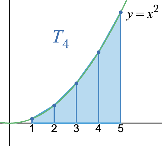
d) Trapezoidal sum

a) Right Riemann sum

1. Divide the interval$[1,5]$ into $n=4$ subintervals, each with equal width:

$$\Delta x=\frac{b-a}{n}$$

$$=\frac{5-1}{4}$$

$$=1$$

This step is the same for all of the sums.

2. Since $n=4$ and this is a right Riemann sum, use the right endpoint of each subinterval to set the rectangle height.

3. The right endpoints are $x=5,4,3,2$ and the function values are:

• $f(5)=25$
• $f(4)=16$
• $f(3)=9$
• $f(2)=4$

4. Then the right Riemann sum is

$$R_4=\Delta x(f(5)+f(4)+f(3)+f(2))$$

$$=1(25+16+9+4)$$

$$=54{\text{ units}}^2$$

b) Left Riemann sum

1. Just as in part a),

$$\Delta x=1$$

2. For a left Riemann sum, use the left endpoint of each subinterval to set the rectangle height.

3. The left endpoints are $x=1,2,3,4$ and the function values are:

• $f(1)=1$
• $f(2)=4$
• $f(3)=9$
• $f(4)=16$

4. Then the left Riemann sum is

$$L_4=\Delta x(f(1)+f(2)+f(3)+f(4))$$

$$=1(1+4+9+16)$$

$$=30{\text{ units}}^2$$

c) Midpoint Riemann sum

1. Just as in the previous parts,

$$\Delta x=1$$

2. The 4 rectangles correspond to these 4 subintervals:

• $[1,2]$
• $[2,3]$
• $[3,4]$
• $[4,5]$

3. For a midpoint sum, the height of each rectangle is the function value at the midpoint of each subinterval.

The midpoint is found by averaging the endpoints. For example,

• Midpoint of $[3,4]=$

$$\frac{3+4}{2}=3.5$$

The midpoints of each subinterval in this example are $x=1.5,2.5,3.5,4.5$ and the function values are:

• $f(1.5)=2.25$
• $f(2.5)=6.25$
• $f(3.5)=12.25$
• $f(4.5)=20.25$

4. Then the midpoint Riemann sum is

$$M_4=\Delta x(f(1.5)+f(2.5)+f(3.5)+f(4.5))$$

$$=1(2.25+6.25+12.25+20.25)$$

$$=41{\text{ units}}^2$$

d) Trapezoidal sum

The area of a trapezoid is

$$A=\frac{h}{2}(b_1+b_2)$$

Here, the trapezoids are oriented sideways:

• the height of each trapezoid is $\Delta x=1$
• the parallel bases have lengths given by the function values at the endpoints of each subinterval

For the leftmost trapezoid, the lengths of the parallel bases are $f(1)$ and $f(2)$.

For the trapezoid next to it, the parallel bases are $f(2)$ and $f(3)$.

Notice that when you add the trapezoid areas, interior function values (like $f(2)$) appear in two adjacent trapezoids, so they get counted twice. Only the endpoint values, $f(1)$ and $f(5)$, are counted once.

Then

$$T_4=\frac{\Delta x}{2}(f(1)+2f(2)+2f(3)+2f(4)+f(5))$$

$$=\frac{1}{2}(1+2(4)+2(9)+2(16)+25)$$

$$=42{\text{ units}}^2$$

Unequal widths

On some AP exam problems, the subinterval widths aren’t all the same, so you can’t use a single $\Delta x$. These problems are often given in a table.

The rate of water, in gallons per minute, flowing into a tank can be modeled by function $g(t)$, which is continuous and strictly increasing on the interval $[0,10]$. Select values are given below:

$t$	$g(t)$
$0$	$3$
$2$	$5$
$5$	$10$
$7$	$12$
$10$	$15$

a) Will a left or right Riemann sum underestimate the actual change in the amount of water?
b) Approximate the net change in the amount of water after 10 seconds using a left Riemann sum with the subintervals$[0,2],[2,5],[5,7],$ and $[7,10]$. Include units.
c) Repeat part b) using a right Riemann sum with the same subintervals. Include units.

Solutions

a) Underestimation

(spoiler)

Because $g(t)$ is strictly increasing, the left-endpoint rectangles lie below the curve on each subinterval. That means a left Riemann sum gives an underestimate of the actual net change. A right Riemann sum uses right endpoints, so its rectangles lie above the curve, giving an overestimate.

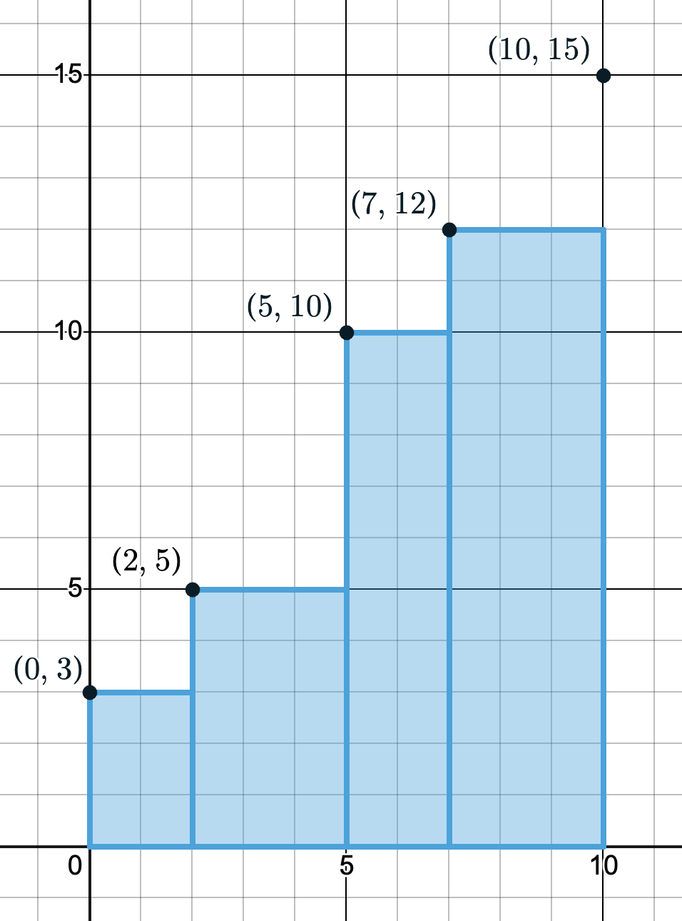
b) Left Riemann sum

(spoiler)

The rectangles can be made as shown in the image below. The units come from multiplying the units of $g(t)$ by the units of $t$, so the result is in gallons.

Use the left endpoint of each subinterval for the height, and use the subinterval length for the width:

• On $[0,2]$: width $2$, height $g(0)=3$
• On $[2,5]$: width $3$, height $g(2)=5$
• On $[5,7]$: width $2$, height $g(5)=10$
• On $[7,10]$: width $3$, height $g(7)=12$

So the approximate net change is:

$$A=2(3)+3(5)+2(10)+3(12)$$

$$=67\text{ gallons}$$

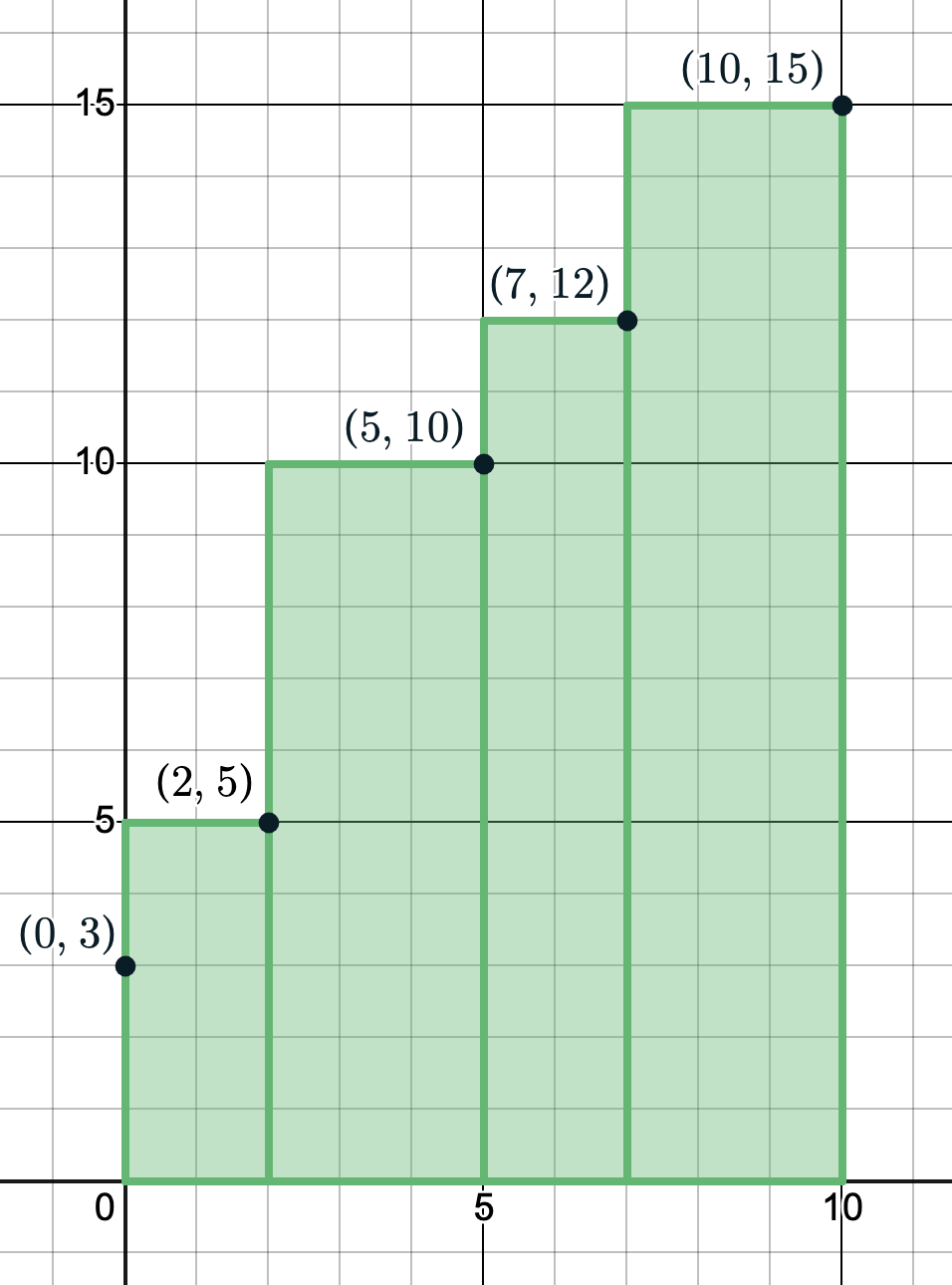
c) Right Riemann sum

(spoiler)

Now use the right endpoint of each subinterval for the height:

The approximate net change is:

$$A=3(15)+2(12)+3(10)+2(5)$$

$$=109\text{ gallons}$$

When deciding whether a Riemann sum is an overestimate or an underestimate, a quick sketch can help you compare the rectangles (or trapezoids) to the curve.

The estimation depends on whether the function is increasing/decreasing (for left/right Riemann sums) or concave up/down (for trapezoidal sums).

• Left sum: If a function is…

  • Increasing $\to$ underestimate
  • Decreasing $\to$ overestimate

• Right sum: If a function is…

  • Increasing $\to$ overestimate
  • Decreasing $\to$ underestimate

• Trapezoidal sum: If a function is…

  • Concave up $\to$ overestimate
  • Concave down $\to$ underestimate