Fundamental theorem of calculus
The previous section showed that derivatives and integrals are opposite processes:
Because integration can “undo” differentiation, when given a function you can look for an antiderivative: a function whose derivative is .
To evaluate a definite integral using this relationship, follow these two steps:
- Find an antiderivative whose derivative is .
- Compute .
The 2nd part of the Fundamental Theorem of Calculus gives a way to evaluate definite integrals:
The notation is a common intermediate step when working with definite integrals. It instructs you to evaluate at the upper limit of integration and subtract its value at the lower limit . You may also see it written with brackets:
Reversing the power rule
Now the question is: how do you find antiderivatives?
Just like with derivatives, there are rules you can use. One of the most important is the reverse power rule. Recall the power rule for derivatives:
To reverse this process for integrals, add to the exponent and divide by the new exponent:
This rule requires (otherwise it would result in division by ). For now, we’ll avoid this case. It will be covered in the next section along with the meaning of .
Example 1: Direct application
Evaluate the definite integral:
Solution
Graphically, the region under from to is a trapezoid with:
-
a height of and
-
parallel base lengths of and .
So we should expect the definite integral to be the area of the trapezoid:
To compute the same value using the FTC, first rewrite with explicit exponents so it’s clear how to apply the reverse power rule:
Apply the reverse power rule term-by-term:
Evaluate :
Using your calculator
While you could use the reverse power rule to evaluate an integral like
doing so by hand takes more time than necessary.
Instead, the calculation can be handled in Desmos with the integral tool:
- Type “int” and an integral symbol will appear.
- Plug in the boundaries.
- Type the integrand.
By entering the integral exactly as shown in the problem, Desmos gives the answer of .
Example 2: Using graphs
The AP Calculus exam frequently tests the FTC using a visual graph instead of a function. In these problems, remember that the definite integral represents the net area under the curve. Calculate these integrals by finding the areas of the geometric shapes formed by the graph.
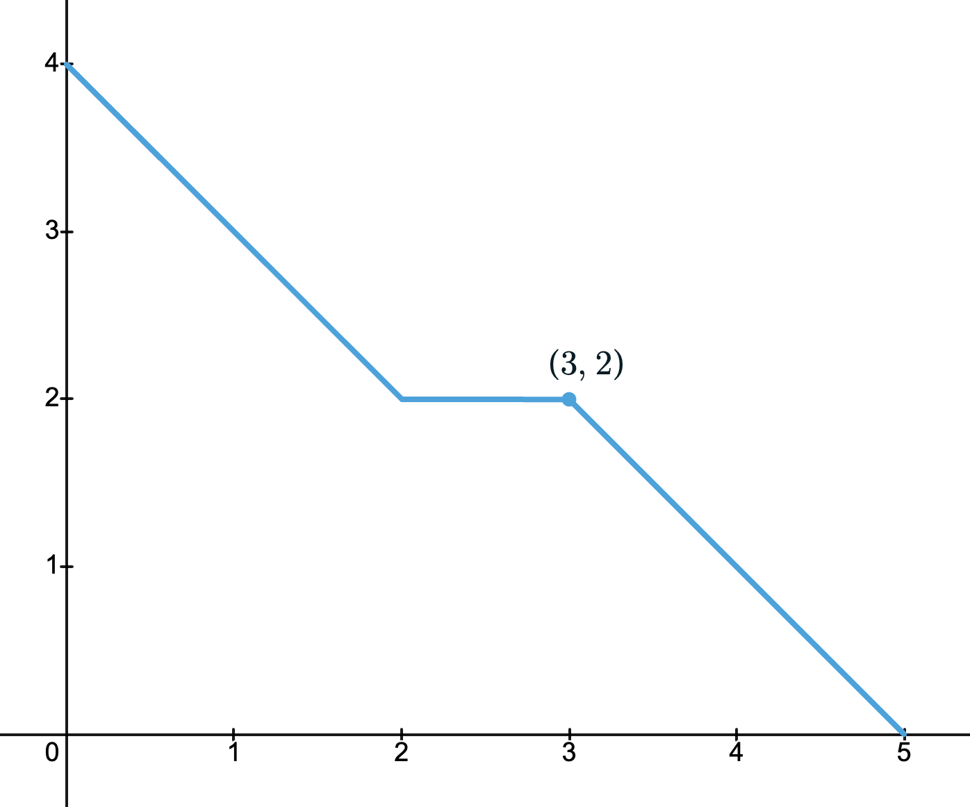
Let be the function whose graph is given below and let be an antiderivative of such that .
a) Find .
b) Find .
c) Find .
Answers
a)
b)
c)
Solutions
a) Find given .
Since is an antiderivative of , we can use the FTC part 2 to evaluate an integral of . The problem gives us and asks for , so setup the integral as follows:
Rearrange to solve for :
Compute the definite integral by finding the net area under the graph from to :
Lastly, substitute into the equation to find :
b) Find .
Since is an antiderivative of , we have by the FTC part 1.
Therefore, . Using the graph of given, locate the function value .
c) Find .
Since , it follows that .
is the slope of the graph of at . Find this by calculating the slope of the line between and :
Example 3: Using tables
A tank contains gallon of water at time . Water is poured into the tank at a rate of gallons per minute, where is measured in minutes. The table below gives values of at selected points:
Use a right Riemann sum with the values in the table to estimate the amount of water in the tank at minutes.
Solution
Let be the amount of water in the tank at time . The problem gives the initial amount of water in the tank, gallon.
Integrating the rate over the time interval from to gives the net change in , or how much water was added:
Solve for :
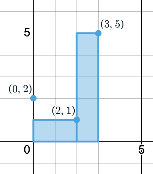
Next, estimate using a right Riemann sum on the subintervals determined by the given -values.
It may help to plot the points and draw the rectangles:
On :
- Width: .
- Height: .
- Area .
On :
- Width: .
- Height: .
- Area .
So the right Riemann sum is , giving the estimate
Then the amount of water in the tank at minutes is