Accumulation functions
An accumulation function is defined using a definite integral with a variable upper limit:
- is a known function (often interpreted as a rate of change).
- is a new function that accumulates the net area from to .
You can think of as the net signed area added between and .
Example
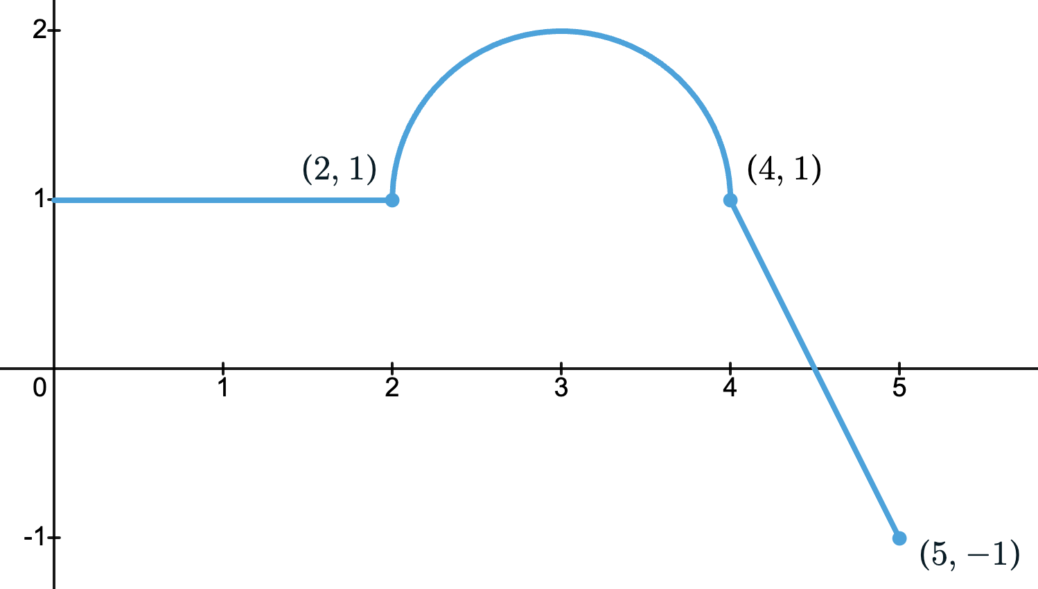
Graphs consisting of piecewise linear segments and standard geometric shapes often appear in the free-response section of the AP exam.
Shown below is the graph of , which consists of two line segments and a semicircle. Let
Find:
a)
b)
c)
Solutions
a)
This integral covers an interval of length , so no area is accumulated.
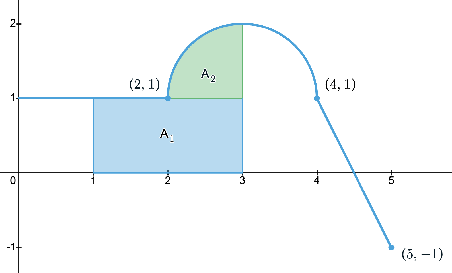
b)
The region under from to consists of:
- A unit rectangle ().
- A quarter-circle of radius ().
Therefore,
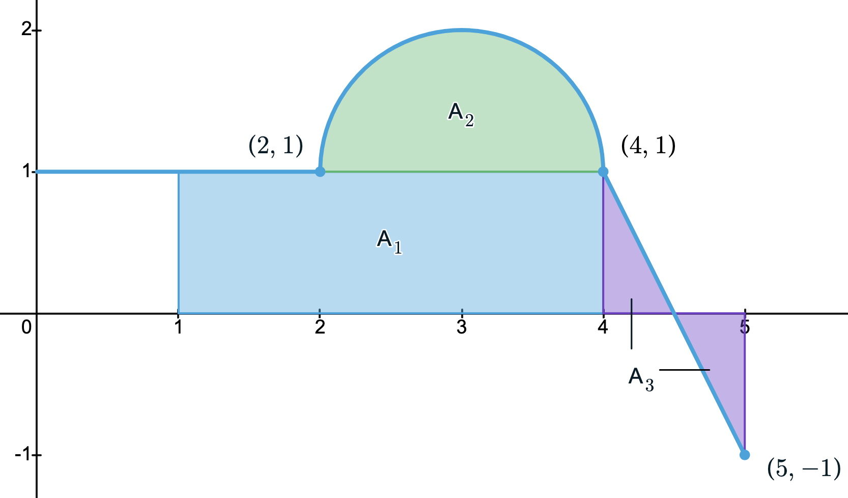
c)
The region from to consists of:
- A rectangle ().
- A semicircle of radius (),.
- Two congruent triangles (one positive, one negative) that cancel each other out ().
Adding the signed areas gives
Fundamental theorem of calculus: part 1
The Fundamental theorem of calculus (FTC), Part 1 establishes that differentiation and integration are inverse operations. Essentially, taking the derivative “undoes” the integral.
When you differentiate , you get back the original integrand, evaluated at the upper limit.
You won’t have to prove this on the AP exam. As long as the lower bound is a real number, you can apply the rule directly: remove the integral, and replace with the upper limit .
A typical problem will be stated as such:
Find given:
Start by writing the derivative:
By the FTC (Part 1), this becomes the integrand evaluated at :
FTC variations (with chain rule)
When the limits of integration are functions instead of a single variable , apply the chain rule. Evaluate the integrand at the upper limit, then multiply by the derivative of that limit.
Variation 1: Functional upper limit
If the upper limit is a function , evaluate the integrand at and multiply by .
Example 1. Find given
Here the upper limit is , so we:
- Replace in the integrand with .
- Multiply by the entire expression by .
Variation 2: Functional lower limit
If the lower limit is a function and the upper limit is a constant, reverse the limits of integration. This introduces a negative sign.
Example 2. Find given
Flip the bounds of the integral and make it negative:
Then, apply the chain rule when differentiating by:
- Replacing every in the integrand with .
- Multiplying the entire expression by its derivative, .
Variation 3: Two variable limits
When both limits are functions of , apply the chain rule to both boundaries and subtract the lower boundary result from the upper boundary result.
Example 3. Find given
Solution
For the upper bound:
- Replace with .
- Multiply by its derivative of .
Subtract the result of the lower bound:
- Replace with .
- Multiply by its derivative of .
Properties of definite integrals
- Splitting an interval
Use this to break up integrals over intervals or to combine pieces.
- Reversing limits
Switching the upper and lower bounds changes the sign.
- Constant multiples
You can factor out constants.
- Linearity
Addition and subtraction work inside integrals.
Given and , find:
a)
b)
Solutions
a) Add over intervals:
b) Reverse the bounds:
Given and , find:
Solution
Using property 1 (splitting up intervals),
Substitute the given values:
Then use property 3 (constant multiples):