Tables and graphs
Limits are the foundational core of calculus. Calculus is the study of change, and limits are what allow us to analyze how a function behaves near a specific point, even if the function is undefined at the point.
Mathematically, a limit describes the value that a function’s output approaches as its input gets closer and closer to a target number.
Understanding limit notation
The limit of as approaches is written as:
This means that as gets closer to , the values of get closer to .
Note that a limit is about what is approaching, not necessarily what equals at . The function value at might be different from , or it might not exist at all.
In fact, does not have to equal or even be defined.
Estimating limits
There are three main ways to evaluate a limit:
- Numerically (from a table)
- Graphically (from a graph)
- Analytically (using algebra or calculus)
This page focuses on the first two methods: estimating limits from tables and graphs.
Limits from a table
One way to estimate a limit is by using a table of values. Choose -values that get closer and closer to from both sides, compute , and look for a value that the outputs seem to settle toward.
Example 1. Estimate based on the table below.
The table shows values of f of x as x approaches 1 from both sides.
As gets closer to , from either side, the values of appear to get closer to , which suggests that
Example 2. Estimate the following limit by creating your own table of values.
Even though is undefined because the denominator is , a limit depends on the values near . So we plug in values of close to into the expression, such as:
As x approaches 2 from either side, the function values approach 5.
From the table, as approaches , the function values approach . So
This matches its graph - the curve approaches a -value of as approaches . Even though is undefined, the limit exists.
Limits that do not exist
There are three common behaviors that lead to a limit that fails to exist. If does any of the following as approaches , then the limit does not exist:
- Oscillates or jumps between values
- Approaches different numbers from the left and right sides
- Increases or decreases without bound (to )
One example of oscillating behavior is
This table shows values of sine of one over x as x approaches 0 from both sides. The outputs oscillate between positive and negative numbers instead of settling on one value.
Despite the symmetry, the output values continue oscillating between positive and negative numbers instead of approaching a single number. Therefore, the limit does not exist.
One-sided limits
Sometimes a function behaves differently depending on whether approaches from the left or from the right. One-sided limits are used to describe these situations, with the following notation:
Left-hand limit:
- Notice the small () above . This means approaches from the left (values smaller than ).
Right-hand limit:
- The small () above means approaches from the right (values larger than ).
For a two-sided limit to exist, both one-sided limits must exist and be equal.
If the one-sided limits are different, then the limit does not exist (DNE).
Based on the table, estimate .
The table shows values of f of x as x approaches 4 from the left and from the right.
As from the left (values smaller than ), appears to approach , suggesting
As from the right (values greater than ), appears to approach , suggesting
Because the one-sided limits don’t match, there is no single value that approaches as . Therefore, does not exist.
Limits from a graph
A graph gives a visual way to track what does as approaches . You can see whether the function approaches a single height, shoots upward or downward without bound, jumps to a different value, or oscillates.
To determine a limit from a graph, follow these steps:
- Follow the graph toward from both the left and the right.
- If approaches the same height from both sides, that height is the limit - even if there is a hole at that point or the function value is elsewhere.
- If approaches different heights from either side, the one-sided limits are different, so the limit does not exist (DNE).
- If increases or decreases without bound, the limit fails to exist in the usual sense but the behavior can still be described using or .
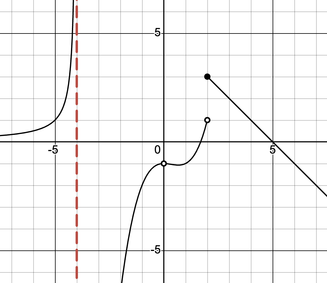
The graph of is shown below with a vertical asymptote at . Based on the graph, find the following limits:
a)
b)
c)
d)
Answers
a)
b)
c) Does not exist
d) Does not exist
Solutions
a)
Although is undefined (a hole indicated by the open circle), the limit depends on what the graph approaches as gets close to . From both sides, the graph approaches . So
b)
The filled-in dot at indicates that
c)
To find the limit, observe how the graph approaches .
- From the left:
As , the graph approaches , so
- From the right:
As , the graph approaches , so
Because these one-sided limits are different, does not exist.
d)
Examine the one-sided limits:
- From the left:
As gets closer to from the left, increases without bound toward . So
- From the right:
As gets closer to from the right, decreases without bound toward . So
Since the one-sided limits don’t match, the overall limit does not exist.