Analytical limits
Evaluating limits analytically
Graphs and tables are usually used when algebraic methods are hard to apply, or as a way to double-check your work. Many limits can be found analytically (using algebra or calculus) with straightforward techniques such as direct substitution and the basic limit laws. Here, you’ll find limits of several types of functions - including piecewise-defined and composite functions - using these analytical methods.
Direct substitution
The simplest way to evaluate a limit is direct substitution. If plugging in into gives a finite number, then that number is the limit.
Always try direct substitution first.
Examples
- Evaluate
Substitute into :
Let’s try another one:
- Evaluate
Solution
Substitute into the expression:
Direct substitution works because these functions are continuous at the point of substitution - meaning . For functions with holes, jumps, or asymptotes at , substitution can fail or give a misleading result.
Limit properties
Direct substitution works in many cases because limits follow a set of rules (limit laws). These laws let you break a complicated expression into simpler pieces.
Some AP-style problems expect you to apply these laws without being given explicit formulas for and . For example:
- Given:
Evaluate:
Use the constant multiple law, the difference law, and the power law to move the limit inside step by step:
Piecewise-defined functions
A piecewise function uses different formulas on different intervals of . When you take a limit at a breakpoint (a value of where the formula changes), you need one-sided limits:
- the left-hand limit (approaching from smaller values)
- the right-hand limit (approaching from larger values)
The overall limit exists only if the two one-sided limits are equal.
Example
Let be the piecewise function defined by
Evaluate:
a) b) c)
Answers
a) Does not exist (DNE)
b)
c)
Solutions
a)
Here, approaches , which is a breakpoint. So we compare the one-sided limits.
- Left-hand limit:
For , the function is , so
- Right-hand limit:
For , the function is , so
Since
the overall limit does not exist.
b)
Here, approaches , which is also a breakpoint.
- Left-hand limit:
For , , so
- Right-hand limit:
For , , so
Both one-sided limits match, so
c)
Since approaches which is not a breakpoint, you don’t need one-sided limits. You just need the correct branch.
Because , we use the third branch, . Therefore,
Composite functions
A composite function is a function inside another function: , also written .
When the outer function behaves nicely (is continuous) at the value the inner function approaches, you can evaluate the limit by working from the inside out.
So the process is:
- Find the limit of the inner function .
- Plug that result into the outer function .
Example
Let and .
Evaluate .
Solution
First, evaluate the inner limit:
Now evaluate at that value:
Challenge problems
The composite-function limit law works when the outer function is continuous at the value approached by the inner function (more on continuity will be covered later).
But what if doesn’t exist, or what if has breaks?
In some cases, finding requires you to evaluate (which may not equal ) when . The multi-part problem below includes several of the trickier cases that can appear on the AP exam, though rare.
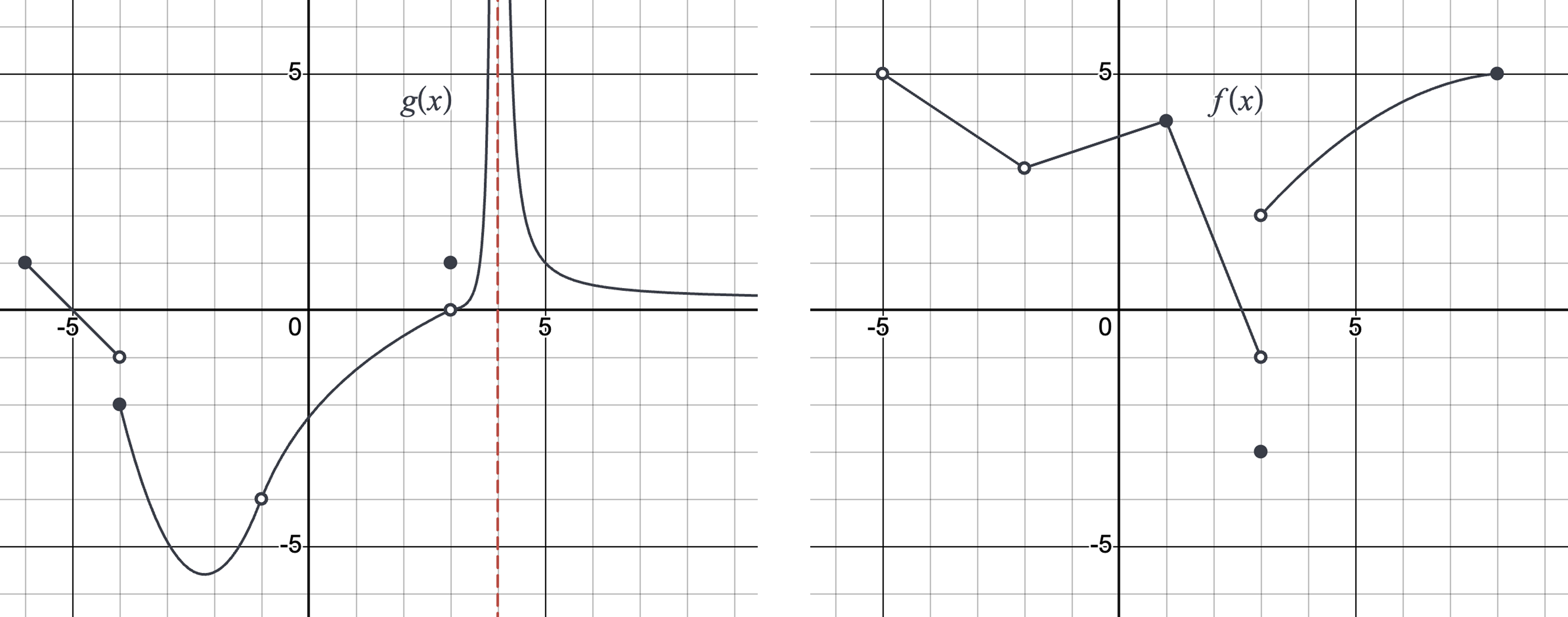
Shown below are the graphs of and :
Evaluate:
a)
b)
Answers
a) DNE
b) (DNE)
Solutions
a)
Start with the inner function:
There is a vertical asymptote at , and both one-sided limits of approach . So does not approach a finite number.
Also, from the graph, the outer function is only defined on the domain . That means the composite can only be evaluated when the output of lands inside that domain.
Since there is no meaningful value for “,” the overall limit does not exist.
b)
First, evaluate the inner limit:
At , the graph of has a vertical asymptote, so it’s reasonable to say the composite limit does not exist.
To be more specific about the behavior:
- As , the graph shows from below (values like , , …).
- Feeding those into , the values , , … grow without bound, consistent with
The same behavior occurs as .
So
which also means the limit does not exist as a finite value.
You can visualize this in Desmos by plotting sample functions with the same local behavior:
- , since
- , since the graph shoots up to on both sides of
- , which will have a vertical asymptote at , so