Continuity
Defining continuity with limits
A function is continuous at a point if and only if it satisfies the following three conditions:
Questions similar to the following have previously appeared on the AP exam:
For what value of will the piecewise function be continuous for all values of ?
For the rational function given, the only point where continuity could fail is at , which is also the breakpoint.
From the piecewise function, .
follows the rational expression for all other values, , so the limit is
Since continuity requires ,
Classifying discontinuities
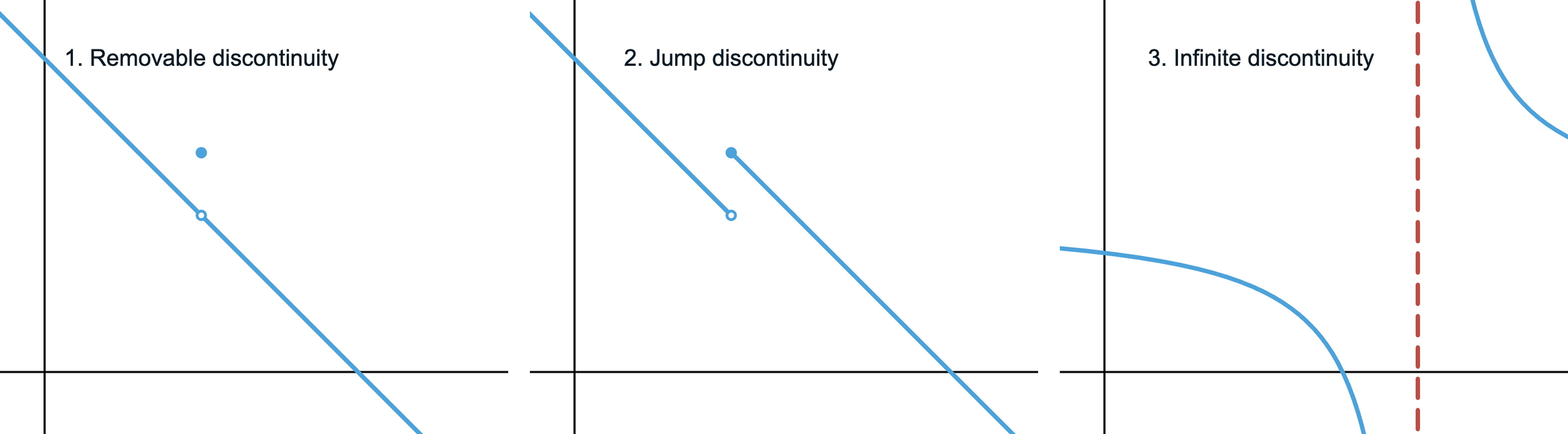
A point that does not satisfy conditions for continuity can be classified into one of three main categories:
1. Removable discontinuity (hole)
- The limit exists but differs from the function value:
- could be undefined or exist as a different value from the limit.
2. Jump discontinuity
- The one-sided limits both exist but differ:
-
“jumps” from one value to another at .
-
Usually seen in piecewise functions at breakpoints.
3. Infinite (asymptotic) discontinuity
- The limit is infinity:
- Means approaches a vertical asymptote at .
Shown below is a visual of each:
Example 1: Rational function
Classify any discontinuities of
1. Find where is undefined
The rational function is undefined when its denominator is :
2. Classify each discontinuity using limits
For :
Direct substitution results in , which indicates a vertical asymptote. The one-sided limits confirm this:
Therefore, there is an infinite discontinuity at .
For :
Since the limit exists but is undefined, there is a removable discontinuity (hole) at .
Example 2: Piecewise function
Let’s explore another example with a piecewise function:
Classify any discontinuities of , where
1. Identify potential discontinuities
Since and are both continuous, the breakpoint is the only point where continuity could fail.
2. Analyze behavior using limits
- Left-hand limit:
- Right-hand limit:
Since the one-sided limits agree, .
However, because the piecewise function defines , then .
Therefore, the discontinuity at is removable.
Challenge problem
Find the values of and such that continuous for all values of .
Each piece is a polynomial that is continuous on its own interval. So the only points where continuity could fail are at the breakpoints of and .
For :
Continuity at requires
The function value is
The one-sided limits must be equal:
For :
Continuity at requires
The function value is
The one-sided limits must be equal:
Now solve the resulting system of equations
which gives and .
Intermediate value theorem
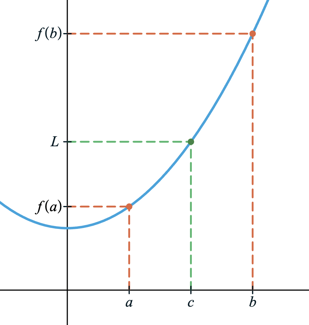
One important consequence of continuity is the Intermediate Value Theorem (IVT).
In plain language, a function that is continuous on can’t “skip over” values. It must take on every -value between and somewhere in that interval.
Examples
Let on the interval . Use the IVT to show that there is a root in the interval.
is a polynomial, which is continuous for all .
A root means (which corresponds to crossing the -axis), so .
Evaluate the endpoints:
Because , the IVT guarantees at least one in such that .
In this particular case, we can confirm by solving :
Only lies within the interval .
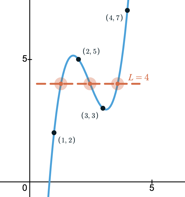
Let be a continuous function defined on the interval . The values of at various points are given in the table:
What is the minimum number of times equals on the interval ?
To find how many times , set the target value to .
It’s often easiest to visualize the situation by sketching a possible graph through the points:
Because the function is continuous, the IVT can be applied to each subinterval. From the table:
-
On , and , and .
-
On , and , and .
-
On , and , and .
So the minimum number of times is times.