



Least squares regression
Least squares regression is a method for finding a line of best fit for a set of data. The goal is to choose the line that makes the sum of the squared vertical differences between the data points and the line as small as possible. Those vertical differences are called residuals.
On the AP Statistics exam, you’ll have a calculator that can compute the least squares regression line from a list of data points. You should know how to do this on your calculator. The short video below shows how to find the line of best fit on a TI-84 (a common calculator for the AP exam), which you’ll use in the next example.
Example 1:
Consider the three points , , . Use the least squares regression method to find the smallest possible sum of the squared errors.
Using the calculator, the line of best fit is:
Next, find each residual (observed minus predicted), square it, and add the results. The original points are , , . The predicted points on the regression line (using the same -values) are , , .
Solution to Example 1:
Thus, the smallest possible value that the sum of squared errors can be is .
Key facts about residuals
- When the data point is above the regression line (i.e. the observed value is greater than the predicted value), then the residual is positive. When the data point is below the regression line (i.e. the observed value is less than the predicted value), then the residual is negative.
- The sum (and mean) of the residuals is always zero.
- The regression line minimizes the sum of the squares of the residuals.
- A residual plot with a nonlinear pattern indicates that a nonlinear model would show a better fit to the data. If there is no apparent pattern or a linear pattern, then a linear model is appropriate.
Practice problem
Part a.
Example 2:
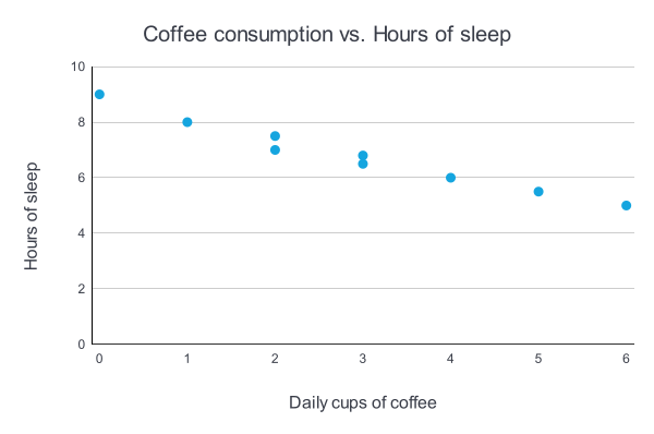
A scientist recorded the coffee drinking habits and sleeping habits of different people, where represents the number of coffee cups that the participant drank each day and represents the number of hours that they sleep each night.
The results were as follows: , , , , , , , , ,
a. What are the explanatory and response variables?
Solution to part a:
The explanatory variable is coffee intake per day () and the response variable is hours of sleep per night ().
Part b.
b. Create a scatter plot.
Solution to part b:
Part c.
c. Describe the relationship as either positive, negative, or neither.
Consider whether hours of sleep tend to increase or decrease as coffee consumption increases.
Solution to part c:
The relationship is negative because, in general, as coffee consumption increases, hours of sleep decrease.
Part d.
d. Use your graphing calculator to find the equation of the regression line.
Use the method shown in the video from Example 1 to find the regression equation.
Solution to part d:
Part e.
e. Interpret the slope in this context.
The slope tells you how (hours of sleep) changes for each one-unit increase in (cups of coffee).
Solution to part e:
For the average participant, sleep decreases by hours for every additional daily cup of coffee consumed.
Part f.
f. Predict how much sleep someone would get who drank cups of coffee.
Substitute into the regression equation.
Solution to part f:
Thus, a person who drank cups of coffee is predicted to have gotten about hours of sleep.