



Aggregate demand
The Aggregate Demand-Aggregate Supply (-) model is the most important model in the course. It is guaranteed to show up many times on the AP Exam, and that is why an entire chapter is spent going over the key pieces of it and discussing how it can be used to evaluate economic scenarios and policy options to address them.
Graphs of this model will have real GDP () on the x-axis and the aggregate price level () on the y-axis. The aggregate price level reflects changes in the overall price level and not changes in relative prices. So increases in represent inflation, decreases in represent deflation.
The GDP deflator is an exact representation of this price level, as it reflects the average price of all goods and services produced in the economy. The CPI, a measure of the average price of goods that consumers buy, may be used as a reasonable approximation.
The aggregate demand curve ( curve) represents total demand in the entire economy. It can be viewed as the total quantity of goods and services that all buyers in an economy are willing and able to purchase at different price levels. “Willing and able” alludes to the fact that at these price levels, the demand curve shows the level of real GDP where spending is equal to income. So for discussions about aggregate demand, it is most natural to interpret real GDP as either spending or income.
This also means that aggregate demand is most easily understood using our GDP equation from earlier in the course. That is,
From this we can separate spending into four major groups of buyers:
- Domestic consumers ()
- Purchases of goods and services (not housing). Depends on disposable income, or income after taxes.
- Businesses ()
- Business investment (capital and inventories), plus housing purchases for consumers
- Government ()
- Purchases of goods and services (including government “investment”).
- Foreign buyers ()
- Foreign purchases minus domestic purchases from foreign production.
The table below illustrates the share of real GDP for each category in 2025.
| C | I | G | NX | |
|---|---|---|---|---|
| Share | 69.2% | 18.6% | 16.7% | -4.5% |
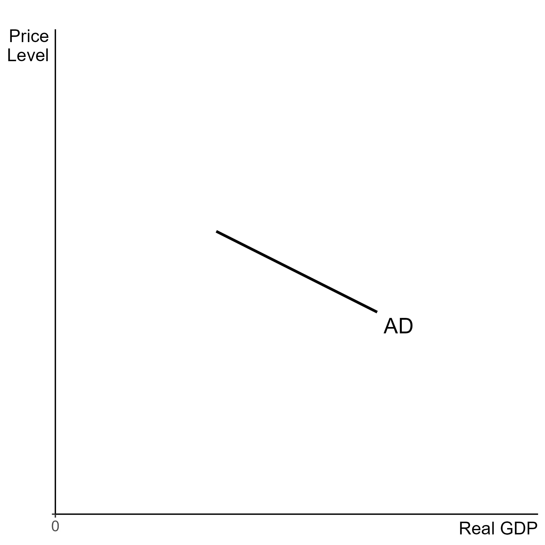
AD graph
Aggregate demand is downward sloping in prices. This is not because of the law of demand, this is the main area where aggregate demand is significantly different from regular demand curves… There are two reasons why the AD curve is downward sloping in prices.
- Wealth effect
- As the price level falls, real income rises. That is, for a given level of income consumers are able to afford to buy a larger amount in real terms. Thus real spending increases. This can be summarized as “people feel richer, so they buy more.”
- Interest rate effect
- When the price level falls, interest rates drop. This makes borrowing cheaper and saving less desirable, so businesses invest more and consumers spend more.
AD shifts
Shifts to aggregate demand include anything that impacts one of the components of GDP. Shifts are always parallel. The slope of the curve does not change.
For any given story it is good to be able to identify which component of GDP is affected, give a one sentence explanation of how it works.
Anything not caused by government policy, spending and taxes, or monetary policy, changes in interest rates, may be referred to as a demand shock.
Consumption and investment
Here are the shifters for consumption and investment.
| Factor Increasing | Change | Impact on |
|---|---|---|
| Household wealth | ||
| Consumer confidence | ||
| Taxes on households | ||
| Interest rates | ||
| Taxes on businesses | ||
| Business confidence |
For every change, if we switch the direction of the change in the factor, the arrow for the impact on is also switched. For example, a fall in household wealth would shift to the left.
Consumption shifts are focused on consumer spending, sometimes referred to as household spending. We have two main factors that lead households to spend more regardless of the price level, increased wealth and increased consumer confidence. Each of these can be thought to be linked to what John Maynard Keynes called the animal spirits, with the bull representing positive sentiment and the bear representing negative sentiment. Bullish signs include a rising stock market, higher expectations for future income and lower uncertainty about the future. Bearish signs include a falling stock market, lower expectations for future income and increased uncertainty about the future.
The stock market is easily tracked, with large amounts of publicly available data on stock prices. Consumer confidence has been tracked for many years using surveys. Two examples are the Conference Board’s Consumer Confidence Index and the University of Michigan’s Index of Consumer Sentiment.
Our final factor that affects mainly households is taxes. Increases in taxes on households, for example income taxes, decrease disposable income, the after-tax income available to be spent or saved. Reduced income has the same effect on consumption as a decrease in wealth, although income should have a larger effect for a similarly sized change.
Interest rate changes impact both households and businesses. Increases in interest rates increase the opportunity cost of consumption today by increasing returns on savings. Thus households save more and consume less. Businesses will also invest less, as higher interest rates reduce the number of projects that they wish to pursue.
Taxes on businesses are generally thought to act similar to taxes on households, only affecting investment instead of consumption. Higher taxes reduce the gains of investment, thus lowering real GDP.
Business confidence is a catch-all for other business specific factors. Confidence includes anything that leads to higher expectations about future profits or reductions in costs. Anticipated increases in demand or reductions in regulations other than taxes are two examples of items that would be expected to increase profits. Technological discoveries or permanent increases in productivity would be examples of cost improvements. In either case, such changes would lead firms to invest more to position themselves to take advantage of better business conditions.
Government
| Factor Increasing | Change | Impact on |
|---|---|---|
| Government spending |
Government spending can be viewed as another source of spending, just like households. So an increase in spending will naturally lead to a rightward shift in the curve. Our usual stories will involve the Federal government, since changes in the spending of a single state or local government will in general not be large enough to move much.
For now this is sufficient, we will discuss other impacts such as how the spending is paid for and potential long-term consequences later on.
Net exports
The final component is net exports ().
| Factor | Change | Impact on |
|---|---|---|
| Foreign income | ||
| Foreign tastes and preferences | ||
| Domestic tastes and preferences | ||
| Exchange rates (non-) |
Increases in foreign income or foreign tastes and preferences for domestic goods, both increase foreign demand for domestic goods. The direct effect is that increases, which lowers and shifts to the right. An increase in domestic tastes and preferences makes fall, which raises and shifts to the right.
Exchange rates are an item that will only be lightly touched upon for now. The exchange rate is only a shifter if it changes for a reason other than changes in the price level. An increase is the same as the dollar getting stronger. That makes exports more expensive for foreigners and imports cheaper in the US. Both changes make fall, and shift to the left.
Consumption and exchange rate dynamics, including how financial flows affect the loanable funds market, will be explored more later on.