



Aggregate supply and equilibrium in the short run
Aggregate supply is where things deviate more significantly from our standard supply and demand stories. There are two versions of aggregate supply, one for the short run and one for the long run. In our final presentation both will be present, along with aggregate demand.
We begin with short run aggregate supply, which is often shortened to . This is an upward sloping curve in the price level and it looks the most like a standard supply curve. Just as with aggregate demand, however, there will be completely different explanations for the slope and new shifts.
The hiring and firing of labor is the primary way to adjust output. Higher real GDP means lower unemployment and lower real GDP means higher unemployment. Thus real GDP has a negative relationship with unemployment. Each will be mentioned as a part of explanations, so this link should be kept in mind.
In the short run, firms decide how much labor to use and how much to produce based on how the observed price level compares to their expectations of the price level. If the price level is equal to the expected price level, then output is , also called potential output. This is equivalent to the economy having an unemployment rate equal to the natural rate of unemployment. As a reminder, that is when cyclical unemployment is zero.
Input prices are also sticky in the short run, so they do not adjust as quickly as output prices. If the price level unexpectedly rises, firms can charge more for their output right away but input costs, for example wages and rent, are temporarily fixed. This expands profit margins, so firms wish to produce more. The concept of sticky prices is the first of our contributions from John Maynard Keynes, who is generally considered to be the father of modern macroeconomics.
If the price level falls, this all occurs in reverse. Output prices fall, but input costs remain the same. This shrinks profit margins, and firms wish to sell less.
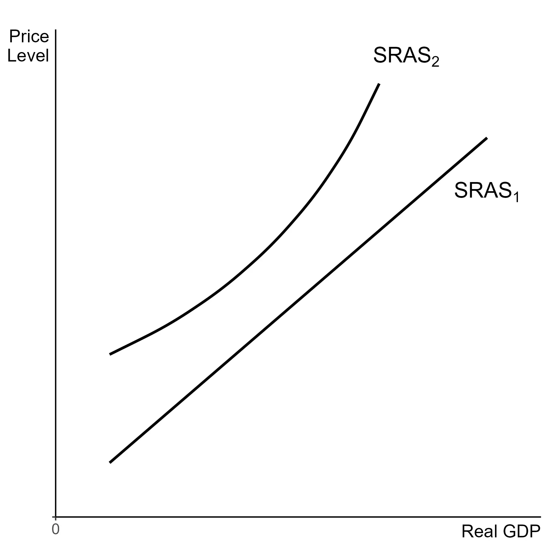
The graph shows the two most standard way to draw a curve. Most examples in the book will draw a straight line, like . A line with some curvature such as is absolutely acceptable as a part of answering free response questions. The key is that it is upward sloping and a not too close to totally vertical or totally horizontal.
In the short run there is a trade-off between the price level and production.
Shifts of only
There are two factors that shift only: inflation expectations and supply shocks.
| Factor | Impact on |
|---|---|
| Positive supply shock | |
| Negative supply shock | |
| Temporarily higher inflation expectations | |
| Temporarily lower inflation expectations |
Supply shocks
A supply shock is any unexpected change that affects production on a large scale. Such changes can be temporary or permanent changes. Any shock that can be expected to go back to the original conditions is temporary. The technical term for this is transitory. These shocks only shift the curve.
Negative shocks can be viewed as increases in costs, either making inputs more expensive or making production less effective. Either way negative shocks raise the real cost per unit of output, and conversely positive shocks lower the real cost per unit of output.
This change shifts to the left (or up). So firms need higher prices to produce every level of real GDP. Equivalently, at every price level we can produce less for the same price.
Examples of transitory negative supply shocks could include
- An increase in oil prices due to an unexpected reduction in production. The tripling of the price of oil from 1973-1975 is a common example.
- The COVID-19 pandemic created shortages in labor and caused an increase in shipping costs.
- A natural disaster, such as a hurricane or drought, that does not cause permanent damage.
Examples of positive supply shocks could include
- A large decrease in the price of raw materials, for example oil or electricity
- An unexpectedly favorable growing season leading to a bountiful harvest
- Temporary business subsidies, such as the CARES Act in response to COVID-19
Inflation expectations
For the AP exam, we are never concerned with how expectations are formed. So understanding why there are changes in inflation expectations is not important. Understanding what happens when they do change is what you are responsible for. There will be some extended examples that will expand on this later.
Shifts due to transitory supply shocks can be thought to include the effects of transitory changes in inflation expectations. Negative supply shocks would lead to temporary increases in expected inflation, and positive supply shocks would lead to temporary decreases in expected inflation.
Outside of a shock, in the short run if inflation expectations change then prices today change in the same direction. So a rise in inflation expectations shifts the curve to the right, making prices higher for every level of production A fall in inflation expectations shifts the curve down, making prices lower for every level of production.
Short run equilibrium
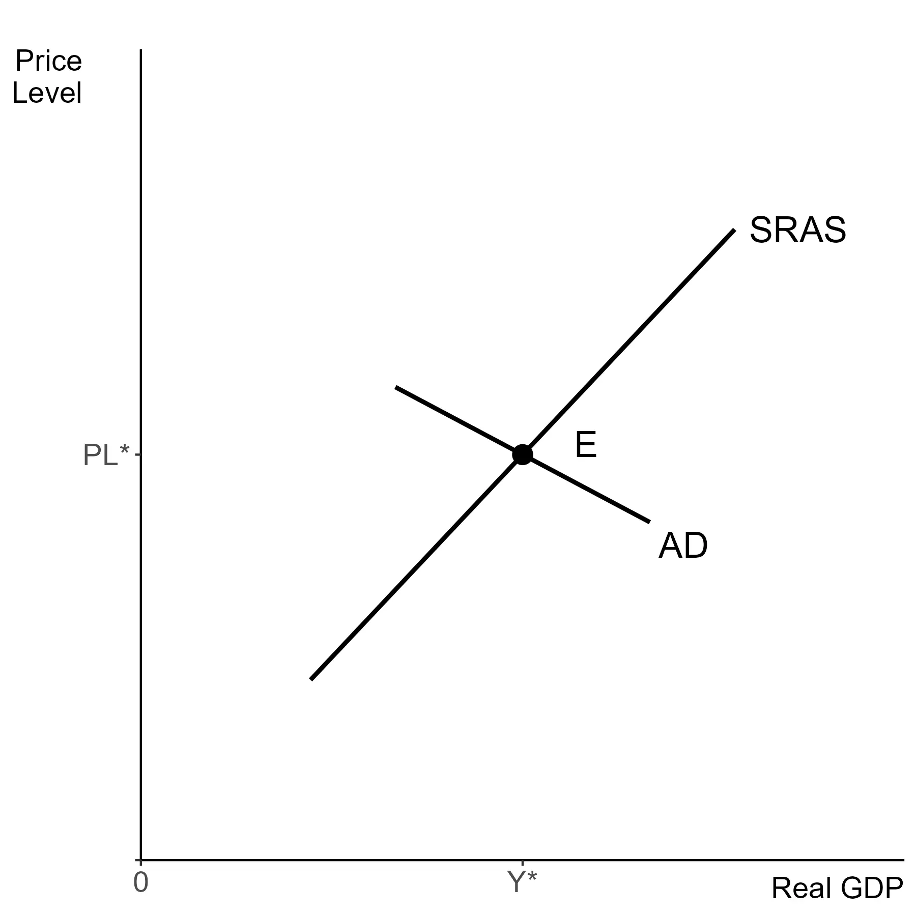
In the short run, equilibrium in the model is determined by the intersection of the aggregate demand curve () and the short run aggregate supply curve (). This sets the price level () and level of real GDP () in the short run
| Shift | Effect on Equilibrium |
|---|---|
Another way to remember this, is that in the short run shifts in aggregate supply move the equilibrium along the aggregate demand curve. Thus and move in opposite directions for those shifts.
On the other hand, shifts in aggregate demand move the equilibrium along the short run aggregate supply curve. In those cases and move in the same direction.