Output gaps and the self adjustment mechanism

Now that we have covered the short run equilibrium and long run equilibrium and how they are affected by shifts in $AD$, $SRAS$ and $LRAS$ we need to connect the two. If any short run change brings us to a place where all three curves cross, then that is the long run equilibrium and there is nothing more of interest.

If not, the intersection of $AD$ and $SRAS$ still gives the short run outcome and the intersection of $AD$ and $LRAS$ still gives the long run outcome. What we need to add are terms to describe these situations and the story of how the short run outcomes transitions into the long run outcome.

Self adjustment mechanism

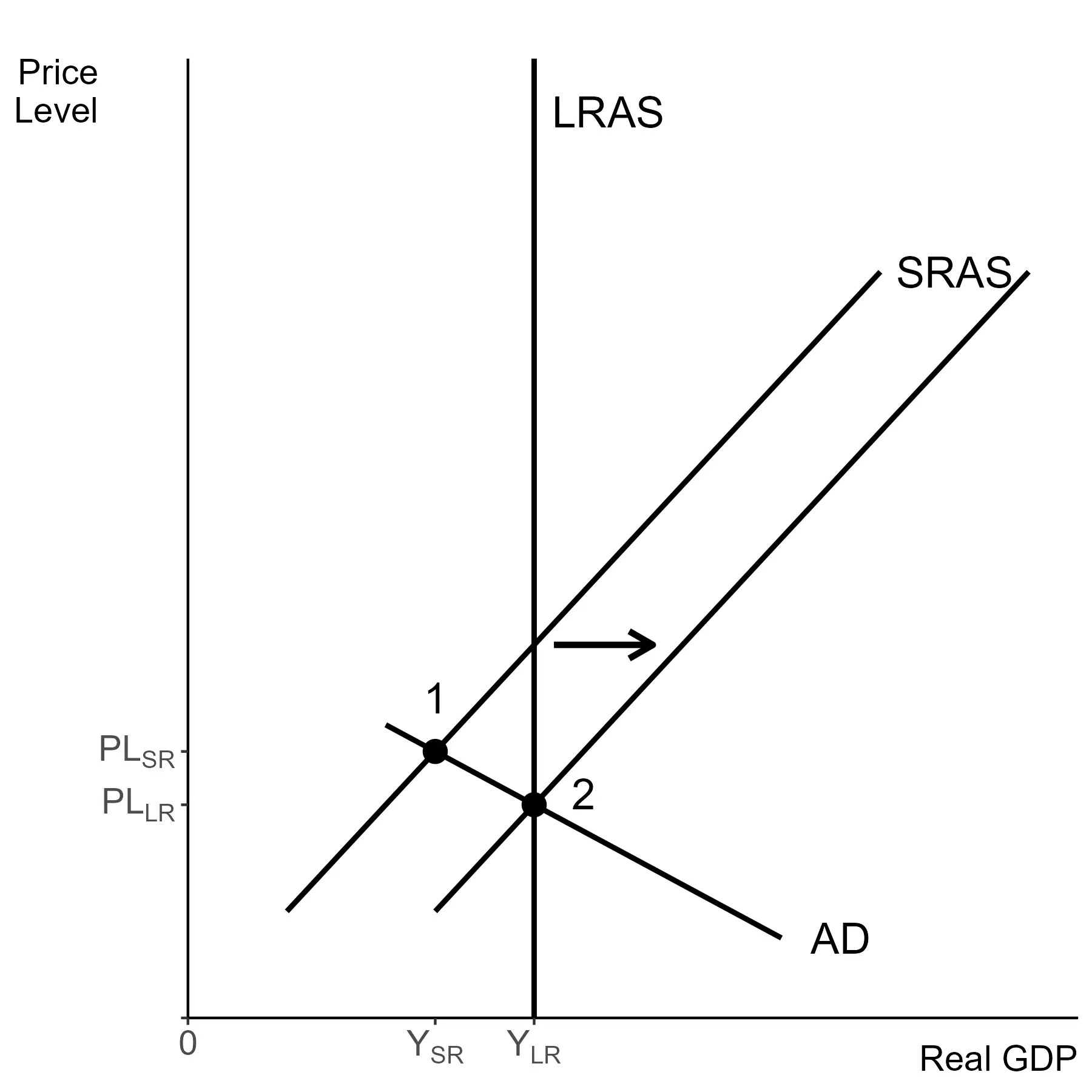
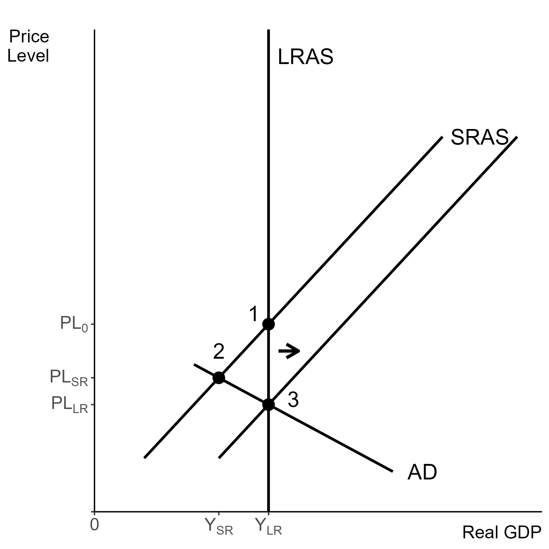
The price level must be equal to the expected price level in the long run, so all three curves need to cross. So what happens if, as in the graph below, the short run equilibrium and long run equilibrium “disagree”?

If the long run equilibrium has higher prices than the short run, higher prices are expected and that leads to the price level rising. Higher expectations mean that workers will negotiate higher wages. Firms realize this will occur and raise their costs, so they raise prices. This shifts the $SRAS$ curve to the right, raising the price level.

Workers will expect a lower price level and accept lower wages. Firms will expect lower wages and that reduction in costs will allow them to lower their prices. This shifts the SRAS curve down (to the left).

If the long run has lower prices than the short run, lower prices are expected and that leads to the price level falling. Workers will expect a lower price level and accept lower wages. Firms will expect lower wages and that reduction in costs will allow them to lower their prices. This shifts the $SRAS$ curve to the left, lowering the price level.

The self-adjustment mechanism is the term for this process. Without policy intervention expectations about inflation are self-fulfilling in the long run. If higher inflation is expected in an economy, that is what happens in the transition to the long run. If lower inflation is expected in an economy, then that is what happens in the transition to the long run.

Recessionary and inflationary gaps

Both of our terms for how the short run relates to the long run end up being fairly intuitively named.

Definitions

Recessionary gap

When real GDP is lower in the short run equilibrium compared to the long run equilibrium. Alternatively, when real GDP is below potential GDP in the short run equilibrium.

Inflationary gap

When real GDP is higher in the short run equilibrium compared to the long run equilibrium. Alternatively, when real GDP is above potential GDP in the short run equilibrium.

Recessionary gap

A recessionary gap corresponds to an economy being in a recession. That requires output below potential GDP in the short run, which means that unemployment is above the natural rate. The difference represents cyclical unemployment. This is represented by point 1 in the graph.

For a recessionary gap the self-adjustment mechanism is for prices to fall, shifting $SRAS$ to the right. This shift moves the economy to point 2, the long run equilibrium where all three curves cross.

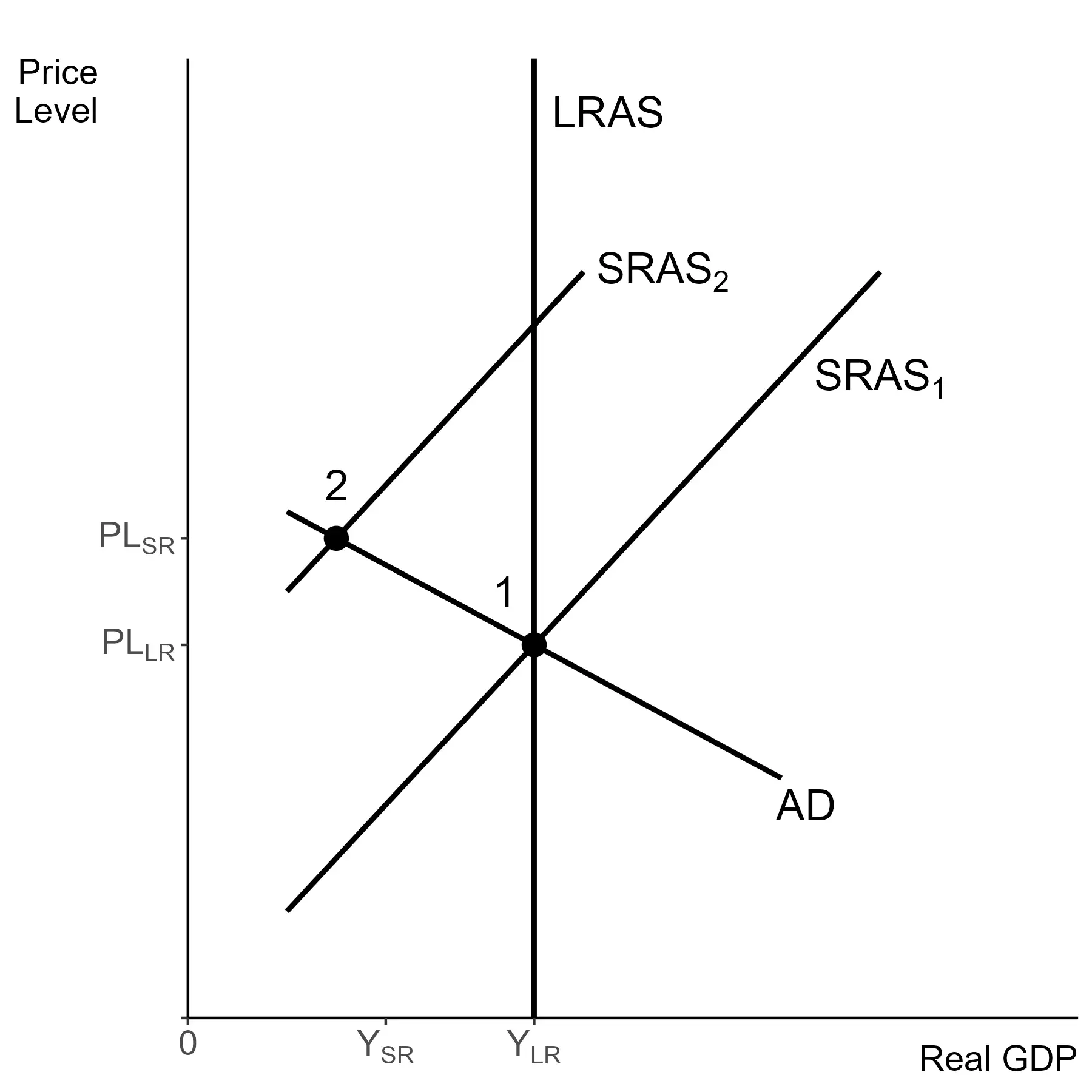
A special case of a recessionary gap is stagflation, a combination of the words “stagnation” and “inflation.” Nearly the only story used is that this is caused by a temporary supply shock, So our initial story is a shift from $SRA{S}_1$ to $SRA{S}_2$, moving our short run equilibrium from point $1$ to point $2$.

Output is below potential, as is the case for any recessionary gap. What makes stagflation special is that it is a significant increase in prices compared to the initial equilibrium. Unemployment rises significantly, and inflation is high as well. This will be a key topic later on.

The self-adjustment mechanism is still the same, the price level falling as expectations of prices fall. This is equivalent to a shift of $SRAS$ back to the original curve and the original equilibrium.

There are definitely costs to larger movements and on a micro level there are likely winners and losers due to the initial unexpected change in the price level. These details are just not accounted for in the $AD$-$AS$ model.

Inflationary gap

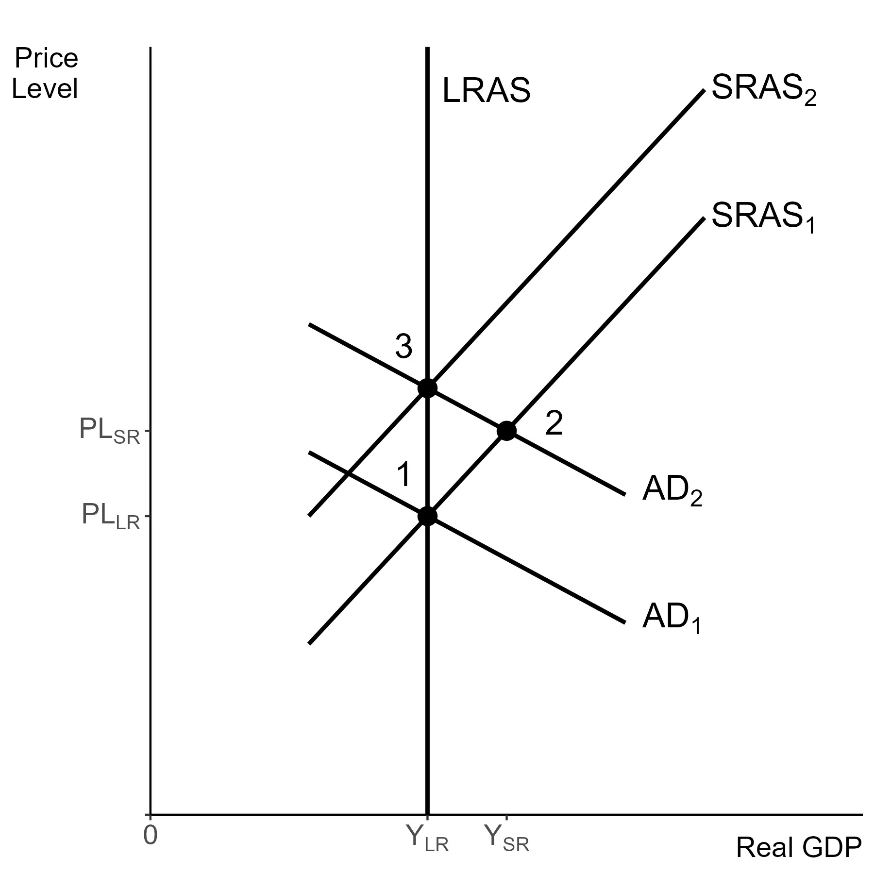
Potential GDP was described as a sort of limit to production for the economy, but that is only strictly true in the long run. In the short run we can temporarily produce more than that level. Consider an economy that starts in long run equilibrium, point $1$. There is a shift in $AD$, for any reason at all, to $A{D}_2$. In the short run the economy moves to point $2$.

Output is higher than $Y^{\star }$, but there is a cost. Initially the cost is that the price level rises, above $P{L}^{\star }$. The self-adjustment response is for the price level to rise further and for output to return to potential output, point 3.

So an inflationary gap leads to inflation now and more inflation in the future, without any permanent gain in real GDP.

Types of inflation

Now that we have laid out the transition from a short run equilibrium to a long run equilibrium, we can categorize inflation by its underlying causes.

Demand-pull inflation is caused by $AD$ shifting so that the short run equilibrium is past $Y^{\star }$. In other words, unemployment is pushed below the natural rate of unemployment.

If we start in long run equilibrium, any increase in $AD$ leads to demand-pull inflation and an increase in the price level in the long run. This fits the inflationary gap graph that was just given.

Anything that shifts $AD$ to the right can cause this, for example an increase in consumer confidence or government spending. This could be the story of 2023, following drops in activity due to the COVID-19 pandemic demand returned to previous levels while supply did not change at the time.

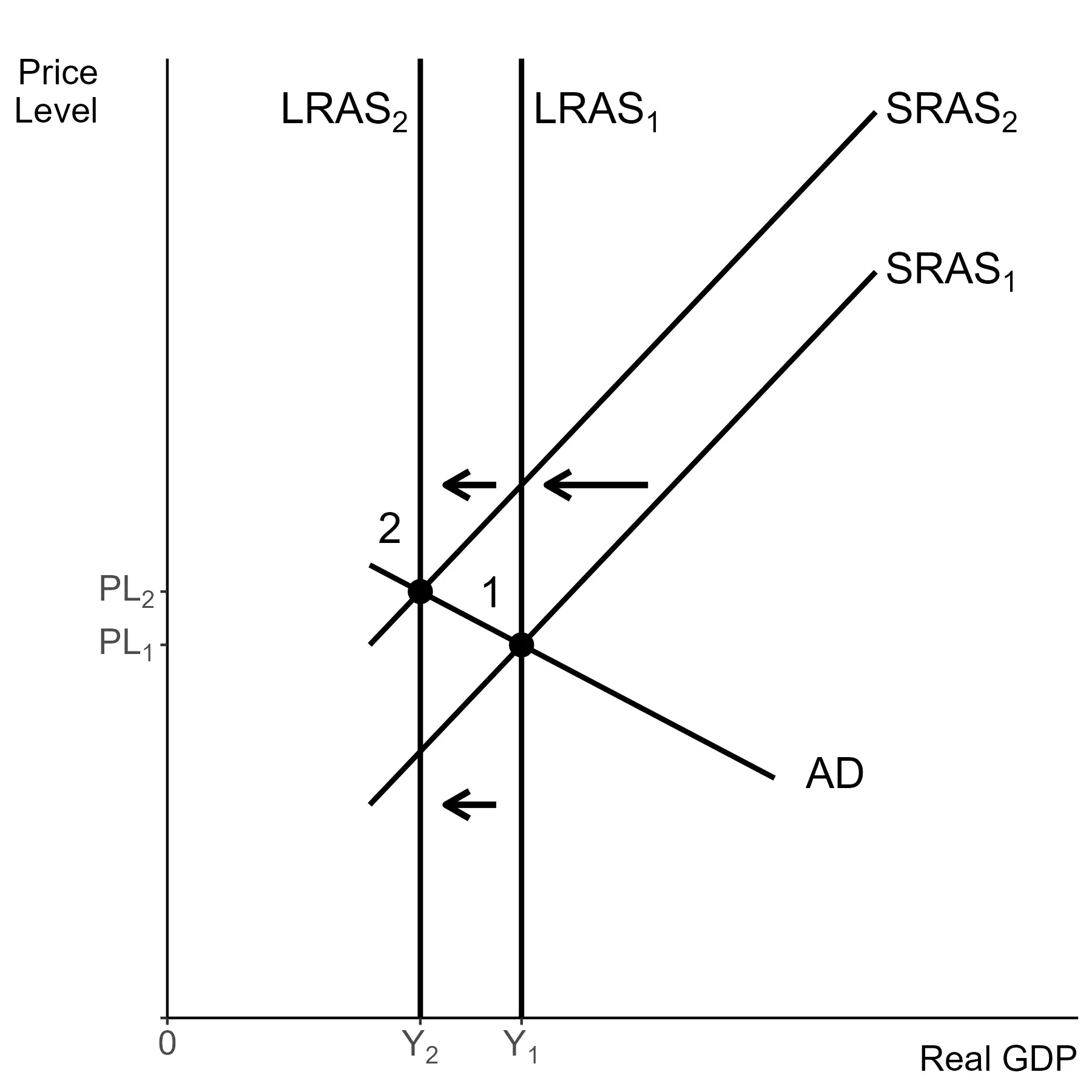
Our second type of inflation is cost-push inflation. This results from rises in input costs, a supply shock. If the supply shock is temporary, the price level rises temporarily and then falls back to the original level in the transition to the long run. In this case inflation is transitory, it rises and then falls again.

Stagflation represents an extreme version of this story. However it is also possible to have smaller shifts in $SRAS$, that do not qualify as stagflation but still lead a temporary rises in costs.

If the supply shock is permanent, then the price level rises and remains higher.

Here the shifts are shown to move the economy directly from one long run equilibrium to another. You may consider equal shifts in the $LRAS$ and $SRAS$, in which case the economy takes two ‘steps’ towards the new long run. A first short run that has a higher price level and lower real GDP, then the new long run that has an even higher price level and an even lower level of real GDP.

FRQs generally allow for any graph that fits the prompt, as long as your explanation is correct. For that reason, a less complicated graph is preferred to a more complicated one. So a multi-step story such as this one should generally be avoided, unless it is directly demanded by the question.

Finally, there is expectations driven inflation. This is a story we have told, but did not label. If workers and firms expect higher prices, wages and prices rise and that leads prices to be higher. This shifts both $AD$ and $SRAS$ to the right.

The expectation of inflation leads to inflation. If there is a continued expectation of inflation, that leads to a wage-price spiral. Expected inflation leads workers to demand higher wages, which leads firms to raise prices.

Then workers expect more inflation and demand higher wages and the cycle repeats. All this story does is lead to shifts in both curves that keep output at potential output, but cause the price level to rise.

Data: the Great Recession

Finally, let us look at the example of the Great Recession, which is dated from December 2007 until June 2009 by the NBER. The table below gives quarterly data on real GDP and the CPI for 2008.

	Q1	Q2	Q3	Q4
Y (billions)	16843	16943	16854	16485
PL (index)	213.45	217.46	218.88	211.40

Real GDP falls for the last two quarters and prices fall in $Q4$. This matches up with what we know about recessionary gaps. Prices falling fits with a recessionary gap due to a fall in $AD$. While the original $AD$ curve is not shown, $Q4$ in the table fits with a movement from point $1$ to point $2$ in the graph. This leaves the economy with a recessionary gap in the short run equilibrium.

We can use what we have learned about the self-adjustment mechanism to predict what will happen in the next year. To return to long run equilibrium, prices need to fall further and real GDP needs to rise (unemployment to fall). Workers accept lower wages, and the corresponding fall in costs allows firms to lower their prices. This shifts $SRAS$ to the left and returns the economy to long run equilibrium at point $3$

In reality, the economy was not allowed to self-adjust. Actions were taken, both monetary and fiscal policy, to try to reduce the negative impacts of the recession. The monetary side will be discussed later. After diving deeper into consumption, we will discuss fiscal policy and review what the US government did in response to this recession.