


Achievable logoAchievable logo
AP Macroeconomics
Sign in
Sign up
Purchase
Textbook
Practice exams
Support
How it works
Exam catalog
Mountain with a flag at the peak
Textbook
Example
1. Core economic concepts
2. Measurement of economic performance
3. Modeling of income and prices
3.1 Aggregate demand
3.2 Aggregate supply and equilibrium in the short run
3.3 Aggregate supply and equilibrium in the long run
3.4 Output gaps and the self adjustment mechanism
3.5 Fiscal policy
3.6 Consumption modeling
3.7 Economic growth
4. Financial sector
5. Long-run consequences of stabilization policy
6. Open economy
Achievable logoAchievable logo
3.3 Aggregate supply and equilibrium in the long run
Achievable AP Macroeconomics
3. Modeling of income and prices
Our AP Macroeconomics course is currently in development and is a work-in-progress.

Aggregate supply and equilibrium in the long run

7 min read
Font
Discuss
Share
Feedback

In the short run, when prices are equal to expected prices then output is equal to potential output, Y⋆. Sticky input prices cause SRAS to be upward sloping in the price level.

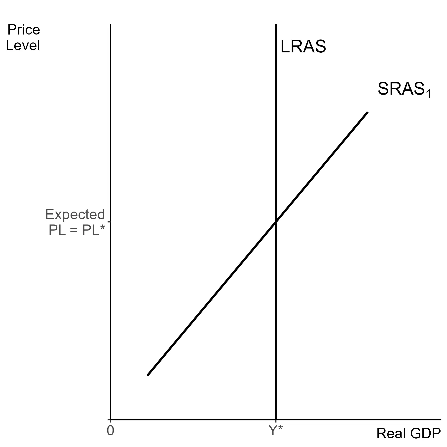
In the long run, all prices have adjusted and there is no longer a trade-off between prices and output. Thus the LRAS line is vertical at Y⋆. This represents the fundamental productive capacity of the economy, the highest level of sustainable production.

Because all prices have adjusted, in the long run the price level must be equal to the expected price level. Connecting back to our original discussion of inflation, that means that in the long run there is no unexpected inflation, there is only expected inflation. No matter what the expectations of prices are, that is where LRAS crosses SRAS.

Vertical aggregate supply in the long run.
Long run aggregate supply

The long run is not a set time frame, but it is widely considered to be between one and three years in most cases. The main point of understanding is that the adjustment period is not fixed, and that for our needs it does not make a major difference exactly how long it is. This transition will be discussed further in the next subchapter.

This is sometimes referred to as the Classical model of supply. All prices adjust immediately, so the economy is always in long run equilibrium. Short run deviations are purely a Keynesian story, which initially were developed as an alternative to the Classical model after the Great Depression…

Shifters of both curves

Every factor that shifts LRAS also causes SRAS to shift in the same direction. Every long run shift may referred to as a supply shock instead of a supply shift.

Factor Impact on LRAS
Technology / productivity LRAS→
Supply of resources LRAS→
Institutions and policy LRAS→

In most cases there is not a strong distinction between technology and productivity. Technology would cover new inventions or the adoption of more advanced production methods, whether they are new or not. Productivity would be anything that permanently increases the amount of output produced by a specific amount of resources or that enables production of the same amount with fewer resources. Either way, it can be viewed as increasing potential output. The economy can produce a higher amount without any increase in inputs.

Weather has been mentioned as a clear example of a temporary supply shock. When it comes to agriculture a permanent shock would be discovery of a new fertilizer or pesticide that increases real output. This increases the level of output we can get for our available inputs, and thus increases the potential GDP of the economy.

The second shifter is an increase in the real resources available to produce. This could either be a higher amount or a higher quality of an input. For macroeconomics the main inputs we consider are labor, capital, raw materials and natural resources, and land. Quality is most easily understood in thinking about the labor force. An increased quality of labor available reflects higher human capital, knowledge and education of the workforce.

Immigration would be one way to increase the available labor force, but if that immigration was targeted towards educated groups, it would have an even larger effect for the same increase in population. This is why many countries have a “points system” for immigration, which may target workers in priority industries and otherwise give points for being healthier and more educated. Being younger is often a plus, as long as you already have a college degree.

Finally, we have institutions and policy choices. This includes nearly all of the role of government, through the outcomes of its investment and spending as well as the limits it places on private markets. Items beyond direct spending often have less clear outcomes. Examples include the enforcement of property rights, the fairness of the court system, the level of corruption, and strictness of regulations for the environment.

A simple example is differences in labor laws, say between France and the United States. In France it is relatively more difficult and more expensive to fire someone and unemployment benefits are more generous. This would be expected to lead to higher frictional unemployment in France, as firms are less willing to hire someone unless they know they have a long term role for them and workers are more able to wait for the “right” fit if they need a new job. This would lead France to have a higher natural rate of unemployment, and thus a lower level of Y⋆.

Government investment would include infrastructure, the basic services and capital expenditures that enable smooth functioning of the economy and the activities of society. Many kinds of infrastructure are considered to be government responsibility, because there are difficulties with provision by private markets. Examples of infrastructure include roads, public transit, airports, sewer systems, electricity and telecommunications grids.

Summary of supply shifts in general

In contrast to temporary supply shocks, as discussed previously, permanent supply shocks shift SRAS and LRAS. The table below briefly summarizes the shifters of aggregate supply. There are no cases where LRAS shifts but SRAS does not.

Factor Change SRAS LRAS
Transitory supply shocks ↑ SRAS← nothing
↓ SRAS→ nothing
Price expectations ↑ SRAS← nothing
↓ SRAS→ nothing
Permanent supply shocks ↑ SRAS← LRAS←
↓ SRAS← LRAS→

An example of a transitory supply shock would be a temporary change in input prices, such as rises in labor costs due to a pandemic or an unexpected spike in oil prices. Permanent supply shocks include changes to technology, productivity, natural resources or institutions.

Long run equilibrium

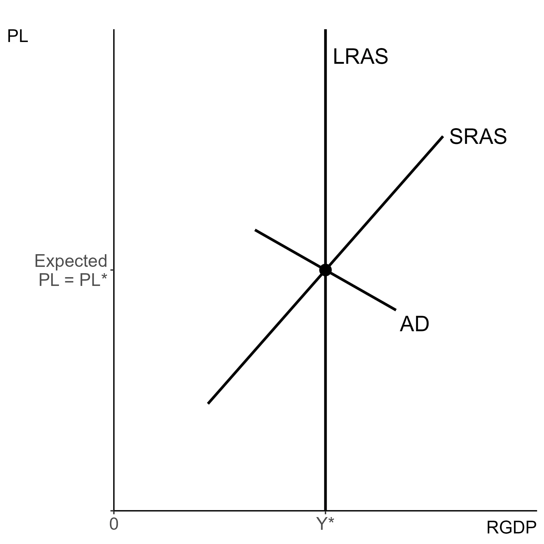
The long run equilibrium is determined by the intersection of the AD curve and the long run aggregate supply (LRAS) curve. In the long run SRAS also needs to cross the AD curve at Y⋆. So all three curves intersect in the long run.

All three curves cross in long run equilbrium.
Long run equilibrium

Recalling that production is equivalent to unemployment, there are three ways to say that the economy is in long run equilibrium.

  1. The price level is equal to the expected price level
  2. Production is equal to potential output
  3. Unemployment is equal to the natural rate of unemployment

What happens when the short run equilibrium and long run equilibrium disagree, will be the next topic.

Previous
Next  | 3.4 Output gaps and the self adjustment mechanism
All rights reserved ©2016 - 2026 Achievable, Inc.

Aggregate supply and equilibrium in the long run

In the short run, when prices are equal to expected prices then output is equal to potential output, Y⋆. Sticky input prices cause SRAS to be upward sloping in the price level.

In the long run, all prices have adjusted and there is no longer a trade-off between prices and output. Thus the LRAS line is vertical at Y⋆. This represents the fundamental productive capacity of the economy, the highest level of sustainable production.

Because all prices have adjusted, in the long run the price level must be equal to the expected price level. Connecting back to our original discussion of inflation, that means that in the long run there is no unexpected inflation, there is only expected inflation. No matter what the expectations of prices are, that is where LRAS crosses SRAS.

The long run is not a set time frame, but it is widely considered to be between one and three years in most cases. The main point of understanding is that the adjustment period is not fixed, and that for our needs it does not make a major difference exactly how long it is. This transition will be discussed further in the next subchapter.

This is sometimes referred to as the Classical model of supply. All prices adjust immediately, so the economy is always in long run equilibrium. Short run deviations are purely a Keynesian story, which initially were developed as an alternative to the Classical model after the Great Depression…

Shifters of both curves

Every factor that shifts LRAS also causes SRAS to shift in the same direction. Every long run shift may referred to as a supply shock instead of a supply shift.

Factor Impact on LRAS
Technology / productivity LRAS→
Supply of resources LRAS→
Institutions and policy LRAS→

In most cases there is not a strong distinction between technology and productivity. Technology would cover new inventions or the adoption of more advanced production methods, whether they are new or not. Productivity would be anything that permanently increases the amount of output produced by a specific amount of resources or that enables production of the same amount with fewer resources. Either way, it can be viewed as increasing potential output. The economy can produce a higher amount without any increase in inputs.

Weather has been mentioned as a clear example of a temporary supply shock. When it comes to agriculture a permanent shock would be discovery of a new fertilizer or pesticide that increases real output. This increases the level of output we can get for our available inputs, and thus increases the potential GDP of the economy.

The second shifter is an increase in the real resources available to produce. This could either be a higher amount or a higher quality of an input. For macroeconomics the main inputs we consider are labor, capital, raw materials and natural resources, and land. Quality is most easily understood in thinking about the labor force. An increased quality of labor available reflects higher human capital, knowledge and education of the workforce.

Immigration would be one way to increase the available labor force, but if that immigration was targeted towards educated groups, it would have an even larger effect for the same increase in population. This is why many countries have a “points system” for immigration, which may target workers in priority industries and otherwise give points for being healthier and more educated. Being younger is often a plus, as long as you already have a college degree.

Finally, we have institutions and policy choices. This includes nearly all of the role of government, through the outcomes of its investment and spending as well as the limits it places on private markets. Items beyond direct spending often have less clear outcomes. Examples include the enforcement of property rights, the fairness of the court system, the level of corruption, and strictness of regulations for the environment.

A simple example is differences in labor laws, say between France and the United States. In France it is relatively more difficult and more expensive to fire someone and unemployment benefits are more generous. This would be expected to lead to higher frictional unemployment in France, as firms are less willing to hire someone unless they know they have a long term role for them and workers are more able to wait for the “right” fit if they need a new job. This would lead France to have a higher natural rate of unemployment, and thus a lower level of Y⋆.

Government investment would include infrastructure, the basic services and capital expenditures that enable smooth functioning of the economy and the activities of society. Many kinds of infrastructure are considered to be government responsibility, because there are difficulties with provision by private markets. Examples of infrastructure include roads, public transit, airports, sewer systems, electricity and telecommunications grids.

Summary of supply shifts in general

In contrast to temporary supply shocks, as discussed previously, permanent supply shocks shift SRAS and LRAS. The table below briefly summarizes the shifters of aggregate supply. There are no cases where LRAS shifts but SRAS does not.

Factor Change SRAS LRAS
Transitory supply shocks ↑ SRAS← nothing
↓ SRAS→ nothing
Price expectations ↑ SRAS← nothing
↓ SRAS→ nothing
Permanent supply shocks ↑ SRAS← LRAS←
↓ SRAS← LRAS→

An example of a transitory supply shock would be a temporary change in input prices, such as rises in labor costs due to a pandemic or an unexpected spike in oil prices. Permanent supply shocks include changes to technology, productivity, natural resources or institutions.

Long run equilibrium

The long run equilibrium is determined by the intersection of the AD curve and the long run aggregate supply (LRAS) curve. In the long run SRAS also needs to cross the AD curve at Y⋆. So all three curves intersect in the long run.

Recalling that production is equivalent to unemployment, there are three ways to say that the economy is in long run equilibrium.

  1. The price level is equal to the expected price level
  2. Production is equal to potential output
  3. Unemployment is equal to the natural rate of unemployment

What happens when the short run equilibrium and long run equilibrium disagree, will be the next topic.

More from Modeling of income and prices

  • Aggregate demand
  • Aggregate supply and equilibrium in the short run
  • Output gaps and the self adjustment mechanism
  • Fiscal policy
  • Consumption modeling