Variables and distributions
Types of variables: Qualitative (categorical) variables are measured on nominal and ordinal scales. Quantitative (continuous) variables are measured on interval or ratio scales.
- Nominal scale: Values are categories with no numerical ranking, such as county of residence, vaccinated or unvaccinated, male or female, etc. A Yes/No variable is also nominal.
- Ordinal scale: Values can be ranked, but the spacing between ranks isn’t necessarily equal, such as stages of cancer. Values are arranged in groups or classes in ascending or descending order (e.g., Stage I breast cancer is less severe than Stage IV).
- Interval scale: Values are measured in equally spaced units, but there’s no true zero point, such as date of birth.
- Ratio scale: This includes interval variables with a true zero point, such as height in centimeters or duration of illness.
Categorical variables are usually summarized as ratios, proportions, and rates. Continuous variables are often summarized with measures of central location and measures of spread.
Frequency distribution:
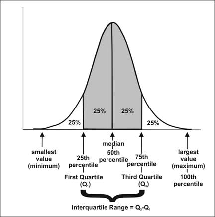
- Normal or symmetric or Gaussian distribution: In this type of frequency distribution, the data cluster around a central value. When plotted, it forms the classic bell-shaped curve. This clustering around a particular value is called the central location (or central tendency) of the distribution. In a normal distribution, the mean, median, and mode are the same.
Bell-shaped curve. The central tendency (the middle) is the median, or 50th percentile. The 25th percentile (the first quartile, Q1) is 25% of the area to the left of the median. The 75th percentile (the third quartile, Q3) is 25% of the area to the right of the median. The interquartile range goes from Q1 to Q3 and makes up 50% of the area under the curve. The largest value is the 100th percentile.
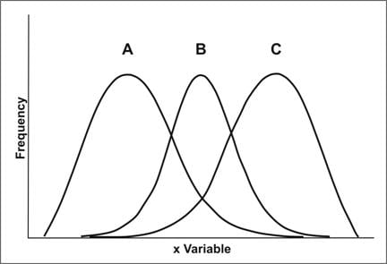
Three superimposed bell curves. The shapes of all three are different. A is shifted to the left. B is symmetrical. C is shifted to the right.
Measures of central location
- Arithmetic mean: The average of all data values. The arithmetic mean is the best descriptive measure for data that are normally distributed. It’s less useful for skewed data because extreme values can pull the mean.
- Median: The middle value after the data have been put into rank order. The median is also the 50th percentile of the distribution.
- Mode: The value that occurs most often in a data set.
- Geometric mean: The mean of data measured on a logarithmic scale. The geometric mean is used when the logarithms of the observations are distributed normally (symmetrically), rather than the observations themselves. It’s useful in microbiological assays.
Problem 1: Calculate the mode from the following data set
1, 1, 2, 2, 2, 3, 3, 3, 3, 3,
Answer is 3 (most common value).
Problem 2: Calculate the median from the following data set
4, 23, 28, 31, 32
Answer is 28 (the middle value).
Problem 3: Calculate the median from the following data set
4, 23, 28, 30, 31, 32
Because the data set has an even number of values, take the average of the middle two values.
In the above example, it will be (28 + 30)/2 = 58/2 = 29.
Problem 4: Calculate the arithmetic mean from the following data set
1, 1, 2, 2, 2, 3, 3
To calculate the mean, add all the values and divide by the number of values.
In the above example: 1+1+2+2+2+3+3 = 14, and 14/7 = 2.
- Asymmetric or skewed distribution: In skewed distributions, the data are not symmetric. Skewness refers to the tail, not the hump. A distribution skewed to the left has a long left tail. A distribution with a central location to the left and a tail extending to the right is positively skewed (skewed to the right). A distribution with a central location to the right and a tail extending to the left is negatively skewed (skewed to the left).
In right skewed distributions, Mode < Median < Mean
In left skewed distributions, Mean < Median < Mode