Standard deviation and confidence intervals
What is spread?
Spread (also called variation or dispersion) describes how data values are distributed around a central value.
Measures of spread include the following:
- Range: The range of a dataset is the difference between its largest (maximum) value and its smallest (minimum) value.
- Quartiles: Data is divided into four equal parts, called quartiles. Each quartile contains 25% of the data. The cut-off for the second quartile is the 50th percentile, which is the median.
- Interquartile range: The interquartile range (IQR) describes the central portion of the distribution, from the 25th percentile to the 75th percentile (i.e., it includes the second and third quartiles).
- Standard deviation (SD or sigma): Standard deviation measures how spread out a dataset is relative to its mean. A lower SD means less variability; a higher SD means more variability. SD is most useful when the data is normally (symmetrically) distributed.
Steps to calculate the SD:
Step 1. Calculate the arithmetic mean.
Step 2. Subtract the mean from each observation.
Step 3. Square each difference.
Step 4. Sum the squared differences.
Step 5. Divide the sum of the squared differences by n − 1.
Step 6. Take the square root of the value obtained in Step 5. The result is the standard deviation.
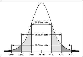
Bell-shaped curve with the standard deviations equally distributed on the x-axis. 99.7% of the data falls between the minus 3 and plus 3 standard deviation. 95.5% of the data falls between the minus 2 and plus 2 standard deviation. 68.3% of the data falls between the minus 1 and plus 1 standard deviations.
Areas included in normal distribution
- ±1 SD includes 68.3%
- ±1.96 SD includes 95.0%
- ±2 SD includes 95.5%
- ±3 SD includes 99.7%
Standard error of mean (SEM): The SEM measures how far the sample mean is likely to be from the true population mean. The SEM is always smaller than the SD.
SEM = Standard deviation/ square root of n, where “n” is the number of observations.
SEM is used to calculate confidence intervals around the arithmetic mean.
Confidence intervals or confidence limits (CI): A confidence interval is a range of values that is likely to contain a population parameter (such as the mean). It is expressed as a percentage (e.g., 95%, 99%).
- The percentage reflects how confident you are that the interval contains the true population mean.
- For example, a 95% confidence interval is a range of values that you can be 95% certain contains the true mean of the population.
- As sample size increases, the interval becomes narrower and precision increases.
- A narrow confidence interval indicates high precision, whereas a wide confidence interval indicates low precision.
CI is given by the formula,
CI = Mean + or - Z x SEM
A CI is reported as a range with a lower and upper limit. For a 95% CI, Z = 1.96. For a 99% CI, Z = 2.58.
Problem 1: Find the 95% confidence interval for a mean total cholesterol level of 206, standard error of the mean of 3.
Using the formula above, upper limit = 206 + 1.96 X 3 = 211.88
Lower limit = 206 - 1.96 X 3 = 200.12
CI is 200.12 to 211.88.
In other words, the best estimate of the true population mean total cholesterol from the given data is 206, but the true mean could reasonably lie anywhere between 200.12 and 211.88.
If the CI of two groups does not overlap, then it means that a statistically significant difference exists. If the CI of two groups overlap, then it means that no significant difference exists.