Direct substitution
Evaluating limits analytically
While creating graphs and tables are excellent tools for visualizing behaviors of functions or double-checking your work, most limits can be evaluated analytically using algebra and calculus. For many functions, straightforward techniques such as direct substitution and the basic limit laws can be used to determine a limit.
Direct substitution
The simplest way to evaluate a limit is direct substitution. If plugging in into gives a finite number, then that number is the limit.
Example 1. Evaluate
Substituting into the expression directly,
Example 2. Evaluate
Substituting directly,
Limit properties
A complicated limit can be broken down into smaller pieces by calculating the limit of each part individually. Limit laws follow standard mathematical rules.
Use these when a specific equation is not given and you must work with graphs or limit values instead.
Examples
Example 1.
Given and , evaluate:
Applying limit laws,
Example 2.
If and , evaluate:
The power law also handles roots since .
Applying limit laws,
Using graphs
Limit laws can also be used after determining limit values from a graph when functions are not explicitly given.
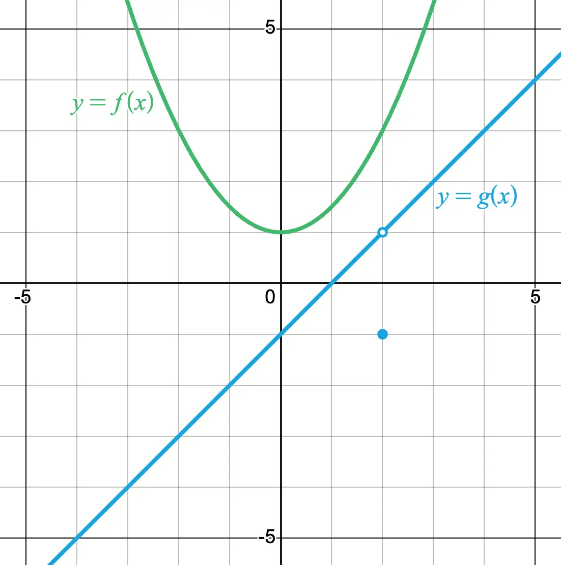
Use the following graphs of and to determine the limits below.
a)
b)
c)
Answers
a)
b)
c)
Solutions
a)
Applying limit laws:
b)
As approaches , the input approaches
So we find the limit of as . From the graph, this limit is .
c)
Apply limit laws to distribute the limit across the terms:
Note: The limit operator only applies to the terms inside the brackets. Because is outside the brackets, it is evaluated separately.
Now evaluate each piece using the graph:
- st term:
As approaches , the input approaches . So we find the limit of as . From the graph, this limit is .
- nd term:
Since , then .
- rd term:
This is a function value, not a limit. Look strictly at the solid dot at , which is at .
Substitute these values back into the expression: