Achievable logoAchievable logo
CMA Part 1
Sign in
Sign up
Purchase
Textbook
Practice exams
Support
How it works
Exam catalog
Mountain with a flag at the peak
Textbook
1. External financial reporting decisions
2. Planning, budgeting, and forecasting
3. Performance management
4. Cost management
5. Internal control
6. Technology and analytics
Achievable logoAchievable logo
3.1.4.4.5 Labor cost variance scenario: Multiple DLs
Achievable CMA Part 1
3. Cost and variance measures
3.1. Management by exception and standard cost systems
3.1.4. Labor cost variance
Our CMA Part 1 course is currently in development and is a work-in-progress.

Labor cost variance scenario: Multiple DLs

8 min read
Font
Discuss
Share
Feedback

Scenario 2: Multiple types of Direct Labor

ChocoDelight Cookies continues its operations with a focus on producing gourmet chocolate chip cookies. To assess production efficiency and cost management, the company now wants to analyze its direct labor performance. The production process involves two types of labor: skilled bakers (Labor A) and assistant bakers (Labor B). Below are the standards and actual data for a recent production batch.

To produce 1,000 cookies, the following usage and cost standards apply:

  • Labor A: 6 hours per 1,000 cookies at $20 per hour
  • Labor B: 4 hours per 1,000 cookies at $10 per hour

Actual results for the recent batch were 1,500 cookies were produced:

  • Labor A: 8 hours at $22 per hour
  • Labor B: 8 hours at $12 per hour

Calculate the Direct Labor variances:

  1. Labor rate variance
  2. Labor efficiency variance
  3. Labor mix variance
  4. Labor yield variance
  5. Labor cost variance

If you would like to check the over-all solution, you can skip to the Scenario summary section at the end of this page.

As discussed previously, the expected production in the master budget of 1,000 cookies will not be very relevant in the computation of the variances as we will focus on the actual production.

Scenario 2.1. Labor rate variance

We need to get the total of the rate variances of each type of direct labor.

Labor Rate Variance Labor A​=(SR×AH)−(AR×AH)=(20×8)−(22×8)=160−176=16(U)​

Alternative computation:

Labor Rate Variance Labor A​=(SR−AR)×AH=(20−22)×8=−2×8=16(U)​

The unfavorable variance of $16 indicates that skilled bakers were paid $2 more per hour than the standard rate, increasing labor costs. Actual Hours (AH) of Labor A is already available at 8 hours and does not need further computations.

Labor Rate Variance Labor B​=(SR×AH)−(AR×AH)=(10×8)−(12×8)=80−96=16(U)​

Alternative computation:

Labor Rate Variance Labor A​=(SR−AR)×AH=(10−12)×8=−2×8=16(U)​

Labor Rate Variance​=Labor Rate Variance Labor A+Labor Rate Variance Labor B=16(U)+16(U)=32(U)​

The total unfavorable variance of $32 reflects higher-than-expected hourly wages for both skilled and assistant bakers, leading to increased overall labor costs.

Scenario 2.2. Labor efficiency variance

The Standard Hours (SH) to be used here is not the one in the master budget but the standard hours that would have been used by the actual production of 1,500 cookies. The following are the SH for both Labor A and B:

SH Labor A=6 hours×(1,500 cookies÷1,000 cookies)=9 hours

SH Labor B=4 hours×(1,500 cookies÷1,000 cookies)=6 hours

We then need to get the total of the efficiency variances of each type of direct labor.

Labor Efficiency Variance Labor A​=(SR×SH)−(SR×AH)=(20×9)−(20×8)=180−160=20(F)​

Alternative computation:

Labor Efficiency Variance Labor A​=(SH−AH)×SR=(9−8)×20=1×20=20(F)​

The favorable variance of $20 shows that skilled bakers worked fewer hours than expected, saving costs.

Labor Efficiency Variance Labor B​=(SR×SH)−(SR×AH)=(10×6)−(10×8)=60−80=20(U)​

Alternative computation:

Labor Efficiency Variance Labor B​=(SH−AH)×SR=(6−8)×10=−2×10=20(U)​

The unfavorable variance of $20 indicates that assistant bakers worked more hours than expected, increasing costs.

Labor Efficiency Variance​=Labor Efficiency Variance Labor A+Labor Efficiency Variance Labor B=20(F)+20(U)=0​

The total efficiency variance of $0 indicates that overall labor hours were consistent with expectations, with favorable savings in skilled labor offset by excess assistant labor hours.

This total efficiency variance can be verified by the computation of the Labor Mix and Labor Yield Variances which will be shown below.

Scenario 2.3. Labor mix variance

When faced with such problems, candidates need to determine the inputs that will be needed in the computations of the variances. Most notably for mix variances, we need to determine the following for each labor used in production:

  • Standard Mix (SM)
  • Actual Mix (AM)
  • Actual Hours Used (AHU)

Standard Mixes (SM), the total of which should be 100%:

SM Labor A=9 hours/(9 hours+6 hours)=60%

SM Labor B=6 hours/(9 hours+6 hours)=40%

Actual Mix (AM), the total of which should be 100%:

AM Labor A=8 hours/(8 hours+8 hours)=50%

AM Labor B=8 hours/(8 hours+8 hours)=50%

Actual Hours Used (AHU) will be total of the actual hours of Labor A (8 hours) and Labor B (8 hours), or 16 hours, used in producing the 1,500 cookies.

Once all the above are determined, we can continue calculating the variances for each type of direct labor.

Labor Mix Variance Labor A​=((AHU×SM)−(AHU×AM))×SR=((16×60%)−(16×50%))×20=(9.6−8)×20=1.6×20=32(F)​

The favorable variance of $32 indicates that fewer skilled baker hours were used compared to the standard mix, reducing labor costs for this category.

Labor Mix Variance Labor B​=((AHU×SM)−(AHU×AM))×SR=((16×40%)−(16×50%))×10=(6.4−8)×10=−1.6×10=16(U)​

The unfavorable variance of $16 reflects that more assistant baker hours were used than expected in the standard mix, increasing overall costs.

Labor Mix Variance​=Labor Mix Variance Labor A+Labor Mix Variance Labor B=32(F)+16(U)=16(F)​

Scenario 2.4. Labor yield variance

We will use the same mixes (SM and AM) computed before.

The Standard Hours Used (SMU) is the total Standard Hours (SH) for both labor types: Labor A (9 hours) + Labor B (6 hours) = 15 hours. Please refer to the Labor Efficiency Variance for explanation of how this was determined.

Labor Yield Variance Labor A​=((SHU×SM)−(AHU×SM))×SR=((15×60%)−(16×60%))×20=(9−9.6)×20=−0.60×20=12(U)​

The unfavorable variance of $12 indicates that the overall labor process required more hours than expected, increasing costs for skilled bakers.

Labor Yield Variance Labor B​=((SHU×SM)−(AHU×SM))×SR=((15×40%)−(16×40%))×10=(6−6.4)×10=−0.40×10=4(U)​

The unfavorable variance of $4 reflects that excess total hours also raised costs for assistant bakers.

Labor Yield Variance​=Labor Yield Variance Labor A+Labor Yield Variance Labor B=12(U)+4(U)=16(U)​

The $16 unfavorable variance highlights inefficiencies in labor utilization, leading to higher-than-expected costs.

We can verify the labor efficiency variance below by adding the mix and yield variances:

Labor Efficiency Variance​=Labor Mix Variance+Labor Yield Variance=16(F)+16(U)=0​

Scenario 2.5. Direct Labor cost variance

The labor cost variance can be computed by adding up the rate and the efficiency variances:

Labor Cost Variance​=Labor Rate Variance+Labor Efficiency Variance=32(U)+0=32(U)​

Alternatively:

Labor Cost Variance Labor A​=(SH×SR)−(AH×AR)=(9×20)−(8×22)=180−176=4(F)​

Labor Cost Variance Labor B​=(SH×SR)−(AH×AR)=(6×10)−(8×12)=60−96=36(U)​

Labor Cost Variance​=Labor Cost Variance Labor A+Labor Cost Variance Labor B=4(F)+36(U)=32(U)​

Scenario summary

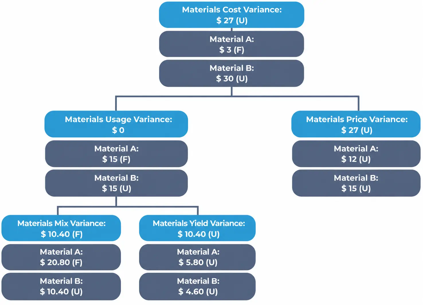
The following illustration shows the summary of the variances for Scenario 2:

With dollar amounts breaking down materials cost variance into usage, price, mix, and yield variances.
Materials Variances Summary

Labor rate variance

  • Measures difference between actual and standard wage rates
  • Both Labor A and B had $2/hour higher rates than standard
  • Total rate variance: $32 Unfavorable (U)

Labor efficiency variance

  • Compares actual hours worked to standard hours for actual output
  • Labor A: 1 hour fewer than standard (Favorable), Labor B: 2 hours more (Unfavorable)
  • Net efficiency variance: $0 (favorable and unfavorable offset)

Labor mix variance

  • Analyzes deviation from standard labor proportion
  • Standard mix: Labor A 60%, Labor B 40%; Actual mix: both 50%
  • Total mix variance: $16 Favorable (F)

Labor yield variance

  • Measures efficiency of total labor hours used versus expected output
  • Actual total hours (16) exceeded standard (15) for 1,500 cookies
  • Total yield variance: $16 Unfavorable (U)

Direct Labor cost variance

  • Overall difference between standard and actual labor cost
  • Sum of rate and efficiency variances
  • Total labor cost variance: $32 Unfavorable (U)

Sign up for free to take 15 quiz questions on this topic

Previous
Next  | 3.1.4.5.1 VOH cost variance summary
All rights reserved ©2016 - 2026 Achievable, Inc.

Labor cost variance scenario: Multiple DLs

Scenario 2: Multiple types of Direct Labor

ChocoDelight Cookies continues its operations with a focus on producing gourmet chocolate chip cookies. To assess production efficiency and cost management, the company now wants to analyze its direct labor performance. The production process involves two types of labor: skilled bakers (Labor A) and assistant bakers (Labor B). Below are the standards and actual data for a recent production batch.

To produce 1,000 cookies, the following usage and cost standards apply:

  • Labor A: 6 hours per 1,000 cookies at $20 per hour
  • Labor B: 4 hours per 1,000 cookies at $10 per hour

Actual results for the recent batch were 1,500 cookies were produced:

  • Labor A: 8 hours at $22 per hour
  • Labor B: 8 hours at $12 per hour

Calculate the Direct Labor variances:

  1. Labor rate variance
  2. Labor efficiency variance
  3. Labor mix variance
  4. Labor yield variance
  5. Labor cost variance

If you would like to check the over-all solution, you can skip to the Scenario summary section at the end of this page.

As discussed previously, the expected production in the master budget of 1,000 cookies will not be very relevant in the computation of the variances as we will focus on the actual production.

Scenario 2.1. Labor rate variance

We need to get the total of the rate variances of each type of direct labor.

Labor Rate Variance Labor A​=(SR×AH)−(AR×AH)=(20×8)−(22×8)=160−176=16(U)​

Alternative computation:

Labor Rate Variance Labor A​=(SR−AR)×AH=(20−22)×8=−2×8=16(U)​

The unfavorable variance of $16 indicates that skilled bakers were paid $2 more per hour than the standard rate, increasing labor costs. Actual Hours (AH) of Labor A is already available at 8 hours and does not need further computations.

Labor Rate Variance Labor B​=(SR×AH)−(AR×AH)=(10×8)−(12×8)=80−96=16(U)​

Alternative computation:

Labor Rate Variance Labor A​=(SR−AR)×AH=(10−12)×8=−2×8=16(U)​

Labor Rate Variance​=Labor Rate Variance Labor A+Labor Rate Variance Labor B=16(U)+16(U)=32(U)​

The total unfavorable variance of $32 reflects higher-than-expected hourly wages for both skilled and assistant bakers, leading to increased overall labor costs.

Scenario 2.2. Labor efficiency variance

The Standard Hours (SH) to be used here is not the one in the master budget but the standard hours that would have been used by the actual production of 1,500 cookies. The following are the SH for both Labor A and B:

SH Labor A=6 hours×(1,500 cookies÷1,000 cookies)=9 hours

SH Labor B=4 hours×(1,500 cookies÷1,000 cookies)=6 hours

We then need to get the total of the efficiency variances of each type of direct labor.

Labor Efficiency Variance Labor A​=(SR×SH)−(SR×AH)=(20×9)−(20×8)=180−160=20(F)​

Alternative computation:

Labor Efficiency Variance Labor A​=(SH−AH)×SR=(9−8)×20=1×20=20(F)​

The favorable variance of $20 shows that skilled bakers worked fewer hours than expected, saving costs.

Labor Efficiency Variance Labor B​=(SR×SH)−(SR×AH)=(10×6)−(10×8)=60−80=20(U)​

Alternative computation:

Labor Efficiency Variance Labor B​=(SH−AH)×SR=(6−8)×10=−2×10=20(U)​

The unfavorable variance of $20 indicates that assistant bakers worked more hours than expected, increasing costs.

Labor Efficiency Variance​=Labor Efficiency Variance Labor A+Labor Efficiency Variance Labor B=20(F)+20(U)=0​

The total efficiency variance of $0 indicates that overall labor hours were consistent with expectations, with favorable savings in skilled labor offset by excess assistant labor hours.

This total efficiency variance can be verified by the computation of the Labor Mix and Labor Yield Variances which will be shown below.

Scenario 2.3. Labor mix variance

When faced with such problems, candidates need to determine the inputs that will be needed in the computations of the variances. Most notably for mix variances, we need to determine the following for each labor used in production:

  • Standard Mix (SM)
  • Actual Mix (AM)
  • Actual Hours Used (AHU)

Standard Mixes (SM), the total of which should be 100%:

SM Labor A=9 hours/(9 hours+6 hours)=60%

SM Labor B=6 hours/(9 hours+6 hours)=40%

Actual Mix (AM), the total of which should be 100%:

AM Labor A=8 hours/(8 hours+8 hours)=50%

AM Labor B=8 hours/(8 hours+8 hours)=50%

Actual Hours Used (AHU) will be total of the actual hours of Labor A (8 hours) and Labor B (8 hours), or 16 hours, used in producing the 1,500 cookies.

Once all the above are determined, we can continue calculating the variances for each type of direct labor.

Labor Mix Variance Labor A​=((AHU×SM)−(AHU×AM))×SR=((16×60%)−(16×50%))×20=(9.6−8)×20=1.6×20=32(F)​

The favorable variance of $32 indicates that fewer skilled baker hours were used compared to the standard mix, reducing labor costs for this category.

Labor Mix Variance Labor B​=((AHU×SM)−(AHU×AM))×SR=((16×40%)−(16×50%))×10=(6.4−8)×10=−1.6×10=16(U)​

The unfavorable variance of $16 reflects that more assistant baker hours were used than expected in the standard mix, increasing overall costs.

Labor Mix Variance​=Labor Mix Variance Labor A+Labor Mix Variance Labor B=32(F)+16(U)=16(F)​

Scenario 2.4. Labor yield variance

We will use the same mixes (SM and AM) computed before.

The Standard Hours Used (SMU) is the total Standard Hours (SH) for both labor types: Labor A (9 hours) + Labor B (6 hours) = 15 hours. Please refer to the Labor Efficiency Variance for explanation of how this was determined.

Labor Yield Variance Labor A​=((SHU×SM)−(AHU×SM))×SR=((15×60%)−(16×60%))×20=(9−9.6)×20=−0.60×20=12(U)​

The unfavorable variance of $12 indicates that the overall labor process required more hours than expected, increasing costs for skilled bakers.

Labor Yield Variance Labor B​=((SHU×SM)−(AHU×SM))×SR=((15×40%)−(16×40%))×10=(6−6.4)×10=−0.40×10=4(U)​

The unfavorable variance of $4 reflects that excess total hours also raised costs for assistant bakers.

Labor Yield Variance​=Labor Yield Variance Labor A+Labor Yield Variance Labor B=12(U)+4(U)=16(U)​

The $16 unfavorable variance highlights inefficiencies in labor utilization, leading to higher-than-expected costs.

We can verify the labor efficiency variance below by adding the mix and yield variances:

Labor Efficiency Variance​=Labor Mix Variance+Labor Yield Variance=16(F)+16(U)=0​

Scenario 2.5. Direct Labor cost variance

The labor cost variance can be computed by adding up the rate and the efficiency variances:

Labor Cost Variance​=Labor Rate Variance+Labor Efficiency Variance=32(U)+0=32(U)​

Alternatively:

Labor Cost Variance Labor A​=(SH×SR)−(AH×AR)=(9×20)−(8×22)=180−176=4(F)​

Labor Cost Variance Labor B​=(SH×SR)−(AH×AR)=(6×10)−(8×12)=60−96=36(U)​

Labor Cost Variance​=Labor Cost Variance Labor A+Labor Cost Variance Labor B=4(F)+36(U)=32(U)​

Scenario summary

The following illustration shows the summary of the variances for Scenario 2:

Key points

Labor rate variance

  • Measures difference between actual and standard wage rates
  • Both Labor A and B had $2/hour higher rates than standard
  • Total rate variance: $32 Unfavorable (U)

Labor efficiency variance

  • Compares actual hours worked to standard hours for actual output
  • Labor A: 1 hour fewer than standard (Favorable), Labor B: 2 hours more (Unfavorable)
  • Net efficiency variance: $0 (favorable and unfavorable offset)

Labor mix variance

  • Analyzes deviation from standard labor proportion
  • Standard mix: Labor A 60%, Labor B 40%; Actual mix: both 50%
  • Total mix variance: $16 Favorable (F)

Labor yield variance

  • Measures efficiency of total labor hours used versus expected output
  • Actual total hours (16) exceeded standard (15) for 1,500 cookies
  • Total yield variance: $16 Unfavorable (U)

Direct Labor cost variance

  • Overall difference between standard and actual labor cost
  • Sum of rate and efficiency variances
  • Total labor cost variance: $32 Unfavorable (U)

More from Labor cost variance

  • Labor cost variance scenario: One type of DL
  • Labor efficiency variances
  • Labor rate variance
  • Overview of labor cost variance formula