Achievable logoAchievable logo
CMA Part 1
Sign in
Sign up
Purchase
Textbook
Practice exams
Support
How it works
Exam catalog
Mountain with a flag at the peak
Textbook
1. External financial reporting decisions
2. Planning, budgeting, and forecasting
3. Performance management
4. Cost management
5. Internal control
6. Technology and analytics
Achievable logoAchievable logo
3.1.3.3.4 Sales variance scenario: multiple products
Achievable CMA Part 1
3. Cost and variance measures
3.1. Flexible budgets
3.1.3. The sales variances
Our CMA Part 1 course is currently in development and is a work-in-progress.

Sales variance scenario: multiple products

7 min read
Font
Discuss
Share
Feedback

Scenario 2: multiple products

The following information is provided for products X and Y for the month of June:

Product X,
budgeted
Product Y,
budgeted
Product X,
actual
Product Y,
actual
Sales volume
(in units)
2,500 3,500 3,000 4,000
Selling price
(in USD)
15 20 17 18

Calculate the following variances:

  1. Total sales variance
  2. Sales price variance
  3. Sales volume variance
  4. Sales mix variance
  5. Sales quantity variance

When faced with a CMA exam problem with multiple products, the best way to calculate the variances is to do them separately for each product and then add them together for the total variance. This example illustrates how to use the different shorthand formulas in computing the variances.

2.1. Total sales variance

The general formula is:

Total sales variance=Actual sales−Budgeted sales

We need to calculate the summation of total sales variance for each product:

Total sales variance product X​=Actual sales product X−Budgeted sales product X=(3,000×17)−(2,500×15)=51,000−37,500=13,500(F)​

Total sales variance product Y​=Actual sales product Y−Budgeted sales product Y=(4,000×18)−(3,500×20)=72,000−70,000=2,000(F)​

Total sales variance​=Total sales variance product X+Total sales variance product Y=13,500(F)+2,000(F)=15,500(F)​

The total sales variance is favorable because the total actual sales are greater than the budget.

2.2. Sales price variance

The general formula is:

Sales price variance​=(Actual selling price−Budgeted selling price)×Actual sales quantity=(ASP−BSP)×ASQ​

We need to calculate the summation of the sales price variances for each product:

Sales price variance product X​=(ASP−BSP)×ASQ=(17−15)×3,000=2×3,000=6,000(F)​

Sales price variance product Y​=(ASP−BSP)×ASQ=(18−20)×4,000=−2×4,000=8,000(U)​

Sales price variance​=Sales price variance product X+Sales price variance product Y=6,000(F)+8,000(U)=2,000(U)​

The sales price variance for Product X is favorable because the actual selling price is higher than budgeted, while it is unfavorable for Product Y because the actual selling price is lower than budgeted. Since the unfavorable variance of Product Y is higher than that of Product X, it results in a net unfavorable variance.

2.3. Sales volume variance

The general formula is:

Sales volume variance​=(Actual sales quantity−Budgeted sales quantity)×Budgeted selling price=(ASQ−BSQ)×BSP​

We need to calculate the summation of the sales volume variances for each product:

Sales volume variance product X​=(ASQ−BSQ)×BSP=(3,000−2,500)×15=500×15=7,500(F)​

Sales volume variance product Y​=(ASQ−BSQ)×BSP=(4,000−3,500)×20=500×20=10,000(F)​

Sales volume variance​=Sales volume variance product X+Sales volume variance product Y=7,500(F)+10,000(F)=17,500(F)​

The sales volume variances for both Product X and Product Y are favorable because the actual units sold are higher than budgeted. This resulted in a total favorable variance.

You can see that the total of the sales price and sales volume variances adds up to the same total sales variance we computed before: 2,000(U)+17,500(F)=15,500(F).

Lastly, the Sales volume variance can be split into the mix and quantity variances, the total of which should agree with the $17,500 favorable variance computed in this section.

Before proceeding, you need to prepare the actual mix % (AM) and standard mix % (SM), which will be used in both mix and quantity variances:

AM % product XAM % product YSM % product XSM % product Y​=3,000+4,0003,000​=42.86%=3,000+4,0004,000​=57.14%=2,500+3,5002,500​=41.67%=2,500+3,5003,500​=58.33%​

2.4. Sales mix variance

The general formula is:

Sales mix variance=((ASQ×AM)−(ASQ×SM))×BSP

We need to calculate the summation of the sales mix variances for each product. Note that the Actual Sales Quantity (ASQ) used here would be the total actual sales quantity of 7,000 units (Product X + Product Y).

Sales mix variance product X​=((ASQ×AM)−(ASQ×SM))×BSP=((7,000×42.86%)−(7,000×41.67%))×15=(3,000−2,917)×15=83×15=1,245(F)​

Sales mix variance product Y​=((ASQ×AM)−(ASQ×SM))×BSP=((7,000×57.14%)−(7,000×58.33%))×20=(4,000−4,083)×20=−83×20=1,660(U)​

Sales mix variance​=Sales mix variance product X+Sales mix variance product Y=1,245(F)+1,660(U)=415(U)​

2.5. Sales quantity variance

The general formula is:

Sales quantity variance=((ASQ×SM)−(BSQ×SM))×BSP

We need to calculate the summation of the sales quantity variances for each product. Note that the Budgeted Sales Quantity (BSQ) used here would be the total budgeted sales quantity of 6,000 units (Product X + Product Y).

Sales quantity variance product X​=((ASQ×SM)−(BSQ×SM))×BSP=((7,000×41.67%)−(6,000×41.67%))×15=(2,917−2,500)×15=417×15=6,255(F)​

Sales quantity variance product Y​=((ASQ×SM)−(BSQ×SM))×BSP=((7,000×58.33%)−(6,000×58.33%))×20=(4,083−3,500)×20=583×20=11,660(F)​

Sales quantity variance​=Sales quantity variance product X+Sales quantity variance product Y=6,255(F)+11,660(F)=17,915(F)​

From here, we can check that the sales volume variance we previously computed with a different approach is equal when we add up the sales mix and quantity variances:

Sales volume variance​=Sales mix variance+Sales quantity variance=415(U)+17,915(F)=17,500(F)​

2.6. Summary

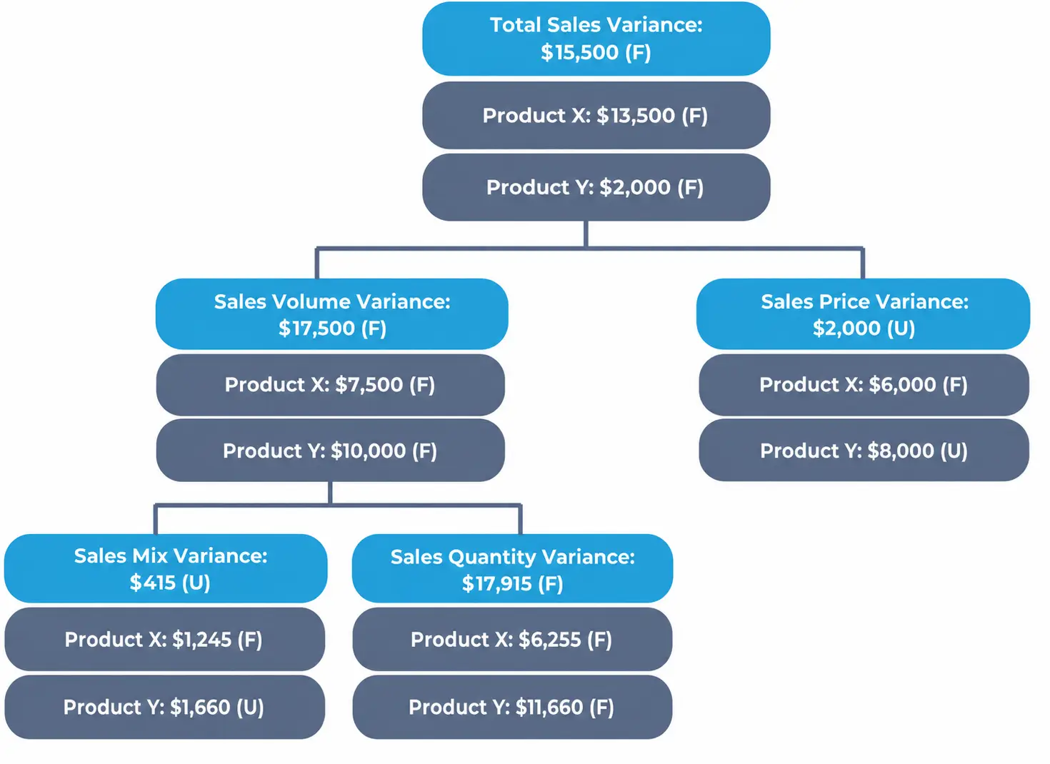
We can summarize all the variance computed from 2.1 to 2.5 into the following illustration:

With dollar amounts breaking down total sales variance by product into volume, price, mix, and quantity variances.
Scenario 2 Sales Variances

Total sales variance

  • Measures difference: actual sales vs. budgeted sales
  • Calculated for each product, then summed
  • Formula: Actual Sales - Budgeted Sales

Sales price variance

  • Measures effect of price changes on sales
  • Formula: (Actual Selling Price - Budgeted Selling Price) × Actual Sales Quantity
  • Favorable if actual price > budgeted; unfavorable if lower

Sales volume variance

  • Measures effect of quantity sold vs. budget
  • Formula: (Actual Sales Quantity - Budgeted Sales Quantity) × Budgeted Selling Price
  • Favorable if more units sold than budgeted

Sales mix variance

  • Measures impact of change in sales mix (proportion of each product sold)
  • Formula: [(Actual Total Sales × Actual Mix %) - (Actual Total Sales × Standard Mix %)] × Budgeted Selling Price
  • Requires calculation of actual and standard mix percentages

Sales quantity variance

  • Measures effect of selling more or fewer units overall, holding mix constant
  • Formula: [(Actual Total Sales × Standard Mix %) - (Budgeted Total Sales × Standard Mix %)] × Budgeted Selling Price
  • Uses total budgeted and actual sales quantities

Key relationships

  • Total sales variance = Sales price variance + Sales volume variance
  • Sales volume variance = Sales mix variance + Sales quantity variance
  • Variances calculated separately per product, then summed for totals

Sign up for free to take 7 quiz questions on this topic

Previous
Next  | 3.1.3.4 The flexible budget variance
All rights reserved ©2016 - 2026 Achievable, Inc.

Sales variance scenario: multiple products

Scenario 2: multiple products

The following information is provided for products X and Y for the month of June:

Product X,
budgeted
Product Y,
budgeted
Product X,
actual
Product Y,
actual
Sales volume
(in units)
2,500 3,500 3,000 4,000
Selling price
(in USD)
15 20 17 18

Calculate the following variances:

  1. Total sales variance
  2. Sales price variance
  3. Sales volume variance
  4. Sales mix variance
  5. Sales quantity variance

When faced with a CMA exam problem with multiple products, the best way to calculate the variances is to do them separately for each product and then add them together for the total variance. This example illustrates how to use the different shorthand formulas in computing the variances.

2.1. Total sales variance

The general formula is:

Total sales variance=Actual sales−Budgeted sales

We need to calculate the summation of total sales variance for each product:

Total sales variance product X​=Actual sales product X−Budgeted sales product X=(3,000×17)−(2,500×15)=51,000−37,500=13,500(F)​

Total sales variance product Y​=Actual sales product Y−Budgeted sales product Y=(4,000×18)−(3,500×20)=72,000−70,000=2,000(F)​

Total sales variance​=Total sales variance product X+Total sales variance product Y=13,500(F)+2,000(F)=15,500(F)​

The total sales variance is favorable because the total actual sales are greater than the budget.

2.2. Sales price variance

The general formula is:

Sales price variance​=(Actual selling price−Budgeted selling price)×Actual sales quantity=(ASP−BSP)×ASQ​

We need to calculate the summation of the sales price variances for each product:

Sales price variance product X​=(ASP−BSP)×ASQ=(17−15)×3,000=2×3,000=6,000(F)​

Sales price variance product Y​=(ASP−BSP)×ASQ=(18−20)×4,000=−2×4,000=8,000(U)​

Sales price variance​=Sales price variance product X+Sales price variance product Y=6,000(F)+8,000(U)=2,000(U)​

The sales price variance for Product X is favorable because the actual selling price is higher than budgeted, while it is unfavorable for Product Y because the actual selling price is lower than budgeted. Since the unfavorable variance of Product Y is higher than that of Product X, it results in a net unfavorable variance.

2.3. Sales volume variance

The general formula is:

Sales volume variance​=(Actual sales quantity−Budgeted sales quantity)×Budgeted selling price=(ASQ−BSQ)×BSP​

We need to calculate the summation of the sales volume variances for each product:

Sales volume variance product X​=(ASQ−BSQ)×BSP=(3,000−2,500)×15=500×15=7,500(F)​

Sales volume variance product Y​=(ASQ−BSQ)×BSP=(4,000−3,500)×20=500×20=10,000(F)​

Sales volume variance​=Sales volume variance product X+Sales volume variance product Y=7,500(F)+10,000(F)=17,500(F)​

The sales volume variances for both Product X and Product Y are favorable because the actual units sold are higher than budgeted. This resulted in a total favorable variance.

You can see that the total of the sales price and sales volume variances adds up to the same total sales variance we computed before: 2,000(U)+17,500(F)=15,500(F).

Lastly, the Sales volume variance can be split into the mix and quantity variances, the total of which should agree with the $17,500 favorable variance computed in this section.

Before proceeding, you need to prepare the actual mix % (AM) and standard mix % (SM), which will be used in both mix and quantity variances:

AM % product XAM % product YSM % product XSM % product Y​=3,000+4,0003,000​=42.86%=3,000+4,0004,000​=57.14%=2,500+3,5002,500​=41.67%=2,500+3,5003,500​=58.33%​

2.4. Sales mix variance

The general formula is:

Sales mix variance=((ASQ×AM)−(ASQ×SM))×BSP

We need to calculate the summation of the sales mix variances for each product. Note that the Actual Sales Quantity (ASQ) used here would be the total actual sales quantity of 7,000 units (Product X + Product Y).

Sales mix variance product X​=((ASQ×AM)−(ASQ×SM))×BSP=((7,000×42.86%)−(7,000×41.67%))×15=(3,000−2,917)×15=83×15=1,245(F)​

Sales mix variance product Y​=((ASQ×AM)−(ASQ×SM))×BSP=((7,000×57.14%)−(7,000×58.33%))×20=(4,000−4,083)×20=−83×20=1,660(U)​

Sales mix variance​=Sales mix variance product X+Sales mix variance product Y=1,245(F)+1,660(U)=415(U)​

2.5. Sales quantity variance

The general formula is:

Sales quantity variance=((ASQ×SM)−(BSQ×SM))×BSP

We need to calculate the summation of the sales quantity variances for each product. Note that the Budgeted Sales Quantity (BSQ) used here would be the total budgeted sales quantity of 6,000 units (Product X + Product Y).

Sales quantity variance product X​=((ASQ×SM)−(BSQ×SM))×BSP=((7,000×41.67%)−(6,000×41.67%))×15=(2,917−2,500)×15=417×15=6,255(F)​

Sales quantity variance product Y​=((ASQ×SM)−(BSQ×SM))×BSP=((7,000×58.33%)−(6,000×58.33%))×20=(4,083−3,500)×20=583×20=11,660(F)​

Sales quantity variance​=Sales quantity variance product X+Sales quantity variance product Y=6,255(F)+11,660(F)=17,915(F)​

From here, we can check that the sales volume variance we previously computed with a different approach is equal when we add up the sales mix and quantity variances:

Sales volume variance​=Sales mix variance+Sales quantity variance=415(U)+17,915(F)=17,500(F)​

2.6. Summary

We can summarize all the variance computed from 2.1 to 2.5 into the following illustration:

Key points

Total sales variance

  • Measures difference: actual sales vs. budgeted sales
  • Calculated for each product, then summed
  • Formula: Actual Sales - Budgeted Sales

Sales price variance

  • Measures effect of price changes on sales
  • Formula: (Actual Selling Price - Budgeted Selling Price) × Actual Sales Quantity
  • Favorable if actual price > budgeted; unfavorable if lower

Sales volume variance

  • Measures effect of quantity sold vs. budget
  • Formula: (Actual Sales Quantity - Budgeted Sales Quantity) × Budgeted Selling Price
  • Favorable if more units sold than budgeted

Sales mix variance

  • Measures impact of change in sales mix (proportion of each product sold)
  • Formula: [(Actual Total Sales × Actual Mix %) - (Actual Total Sales × Standard Mix %)] × Budgeted Selling Price
  • Requires calculation of actual and standard mix percentages

Sales quantity variance

  • Measures effect of selling more or fewer units overall, holding mix constant
  • Formula: [(Actual Total Sales × Standard Mix %) - (Budgeted Total Sales × Standard Mix %)] × Budgeted Selling Price
  • Uses total budgeted and actual sales quantities

Key relationships

  • Total sales variance = Sales price variance + Sales volume variance
  • Sales volume variance = Sales mix variance + Sales quantity variance
  • Variances calculated separately per product, then summed for totals

More from The sales variances

  • Sales variance scenario: one type of product
  • Sales volume variance
  • Total sales variance and sales price variance