


Achievable logoAchievable logo
CMA Part 1
Sign in
Sign up
Purchase
Textbook
Practice exams
Support
How it works
Exam catalog
Mountain with a flag at the peak
Textbook
1. External financial reporting decisions
2. Planning, budgeting, and forecasting
3. Performance management
4. Cost management
5. Internal control
6. Technology and analytics
Achievable logoAchievable logo
3.1.3.4 The flexible budget variance
Achievable CMA Part 1
3. Performance management
3.1. Cost and variance measures
3.1.3. Flexible budgets
Our CMA Part 1 course is currently in development and is a work-in-progress.

The flexible budget variance

7 min read
Font
Discuss
Share
Feedback
Definitions
Flexible budget variance
A variance that measures the difference between actual results and the flexible budget.

We can use the following general formula as guidance:

Flexible budget variance=Actual results−Flexible budget

This calculation is applied to all key line items, including revenues, variable costs, fixed costs, and operating profit. Since the quantities are constant between the actual results and the flexible budget, managers can isolate variances attributable to factors such as price changes, efficiency, and cost control. These variances provide insight into operational efficiency, pricing strategies, and cost management, helping managers pinpoint areas requiring attention.

It can be observed that the flexible budget variance is actually computed the same way as the price variance. If a CMA problem asks to compute the flexible budget variance, you can remember the formula for the price variance in order to arrive at the answer.

Flexible budget variance analysis

Flexible budget variance analysis extends beyond a single line item, such as sales revenue, to examine the entire income statement. This approach provides a more comprehensive view of an organization’s financial performance, allowing managers to identify and address variances across multiple categories, including costs and profitability.

We already had a discussion about the flexible budget variance in the earlier chapter which showed a simplified scenario where only sales and production volume changed while prices did not. This section would expand further the implications in the examination of when volume, sales prices and input prices have deviated from the budget.

Example analysis

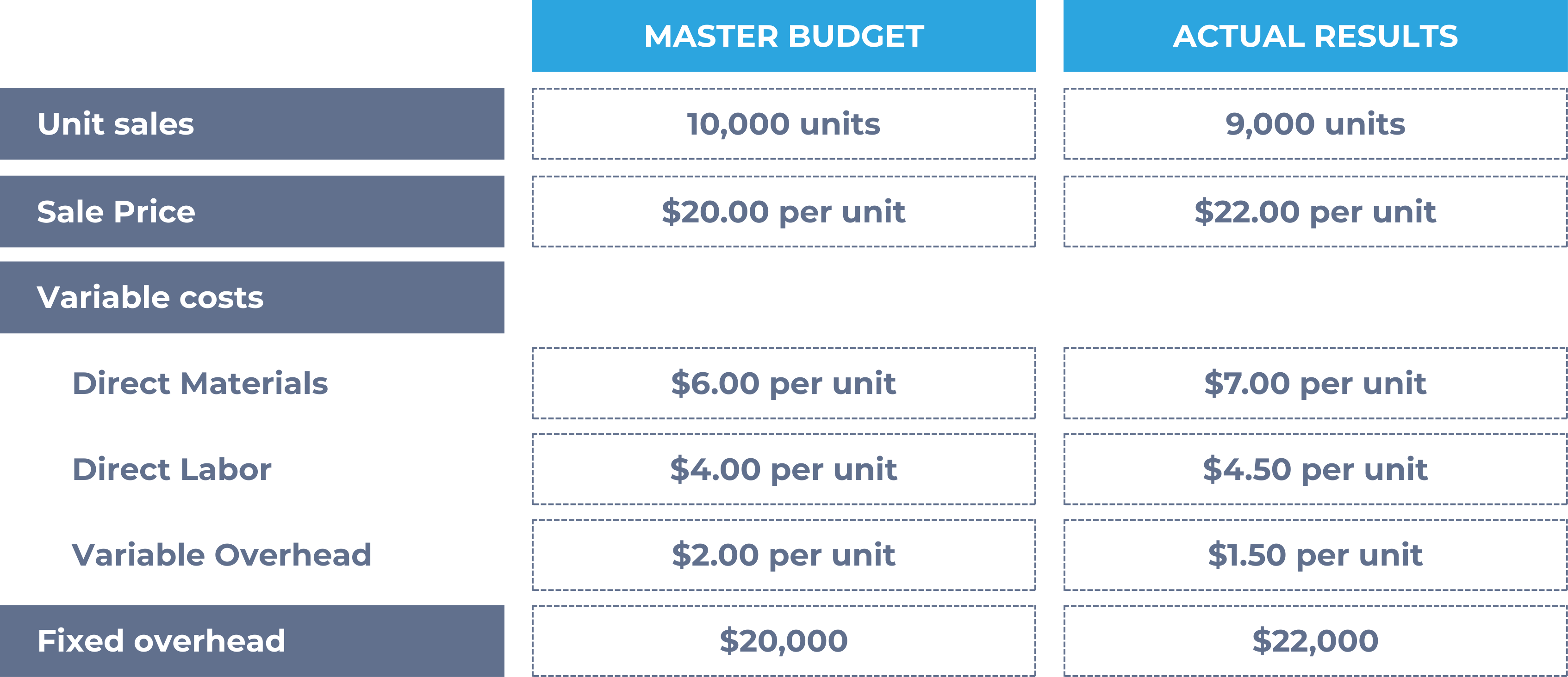
Consider the following example company that has the following budgeted and actual results:

Flexible budget exercise

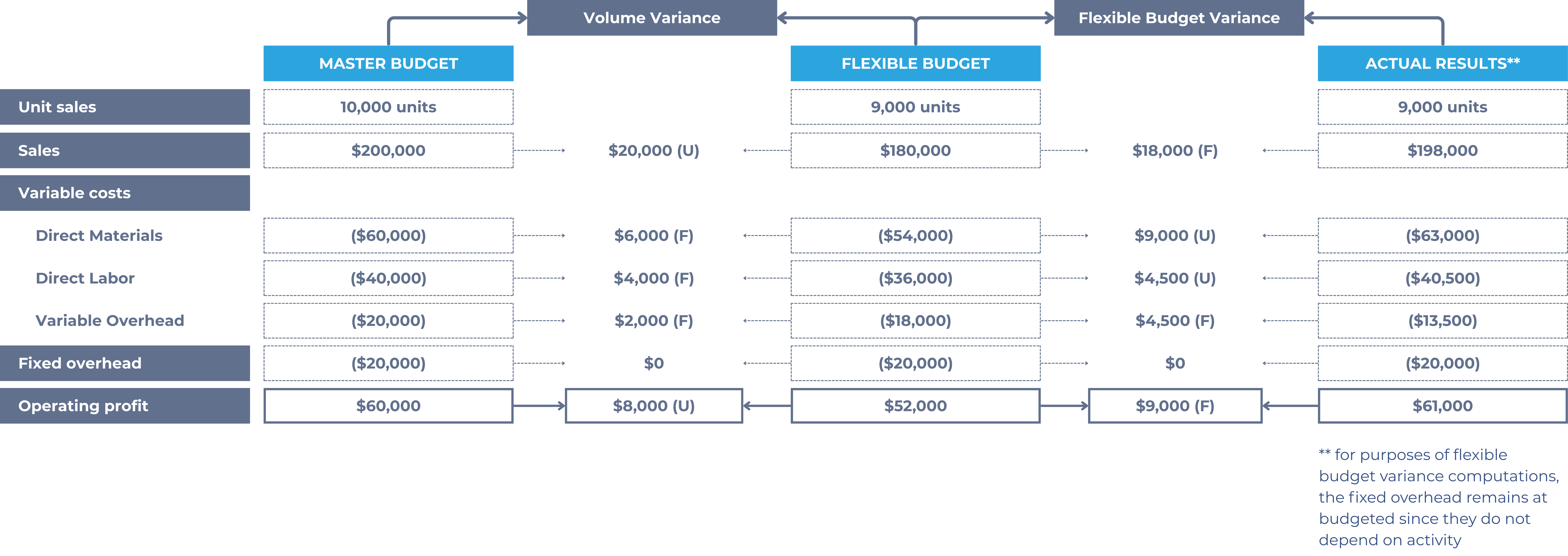
We can prepare the flexible budget by adjusting the master budget of the actual units sold (9,000). We can then examine the flexible budget variance by comparing the actual results to the flexible budget.

Flexible budget exercise - total variance

The analysis shows a total flexible budget variance of $9,000 favorable based on operating profit. While this figure indicates that actual performance was slightly better than expected overall, it does not provide meaningful insight on its own. The total variance must be broken down into its individual components, such as revenue, direct materials, direct labor, and overhead, in order to understand the underlying reasons for the difference.

1. Revenue variances

The total unfavorable revenue variance of $2,000 is explained by:

  • A favorable sales price variance of $18,000, resulting from the actual sales price of $22 per unit, which exceeded the budgeted price of $20 per unit, reflecting successful pricing strategies or favorable market conditions. This sales price variance is the same as the flexible budget variance for sales.
  • An unfavorable sales volume variance of $20,000, due to selling 9,000 units instead of the budgeted 10,000 units, which could indicate lower demand, production constraints, or external market factors.

For further insights into these variances, refer to the detailed discussions on sales price and sales volume variances in the previous section.

2. Direct material flexible budget variance

The flexible budget variance for direct materials is $9,000 (U), indicating that the company spent more on materials than expected based on the actual production volume.

The flexible budget cost for direct materials was $54,000 (9,000 units × $6 per unit), while the actual cost was $63,000 (9,000 units × $7 per unit). This means the company spent $1 more per unit than budgeted, resulting in the unfavorable variance.

There are several potential reasons for this variance. The cost increase could be due to higher material prices driven by market conditions, such as inflation or supply chain disruptions. Inefficient procurement practices, such as last-minute purchases or reliance on higher-cost suppliers, might also have contributed. Alternatively, the variance could reflect a strategic choice to use higher-quality materials, which would improve the product but at a higher cost. Waste or scrap during production could further exacerbate the unfavorable variance, suggesting inefficiencies in material usage or handling.

3. Direct labor flexible budget variance

The flexible budget variance for direct labor is $4,500 (U), reflecting higher-than-expected labor costs.

Based on the flexible budget, direct labor costs were expected to be $36,000 (9,000 units × $4 per unit), but actual costs amounted to $40,500 (9,000 units × $4.50 per unit). This variance indicates that the company spent $0.50 more per unit on labor than planned, resulting in higher overall costs for the actual production volume.

Several factors could have contributed to this unfavorable variance. Increased hourly wage rates, possibly due to overtime, labor shortages, or higher negotiated pay rates, could account for the cost increase. Lower productivity levels might have required more hours to produce the same number of units, raising costs despite budgeted expectations. Additional factors, such as hiring less experienced staff who required more training or supervision, could also lead to inefficiencies in labor usage. Alternatively, external market conditions, such as inflation or competition for skilled workers, may have driven up labor costs.

4. Variable overhead flexible budget variance

The flexible budget variance for variable overhead is $4,500 (F), indicating that actual variable overhead costs were lower than expected based on the actual production volume.

The flexible budget allocated $18,000 for variable overhead (9,000 units × $2 per unit), but actual costs were only $13,500 (9,000 units × $1.50 per unit). This favorable variance reflects savings of $0.50 per unit, reducing overall costs compared to the budgeted amount.

The specific reasons for this favorable variance depend on the nature of the variable overhead expenses, which were not detailed in this example. Common types of variable overhead include utilities, indirect materials, and maintenance costs. Lower-than-expected costs might result from improved efficiency, such as reduced machine run time leading to savings in energy consumption or lower maintenance requirements. Effective resource management, such as minimizing waste of indirect materials or streamlining production processes, could also contribute to the favorable variance.

5. Fixed overhead flexible budget variance

The flexible budget variance for fixed overhead is zero, because fixed costs are assumed to remain constant regardless of the level of production. In the flexible budget, the fixed overhead is held at the budgeted amount of $20,000, and this same figure is used when comparing against actual production volume.

Although the actual fixed overhead incurred was $22,000, this difference does not appear in the flexible budget variance analysis. By design, the flexible budget focuses only on the impact of changes in activity level, and therefore assumes that fixed costs do not increase or decrease with changes in volume. Any variance between the actual and budgeted fixed costs, such as the $2,000 excess in this case, is analyzed separately through other variance categories (e.g., fixed overhead spending variance), not within the flexible budget variance framework.

This approach reinforces the principle that fixed overhead costs should not vary with output in the short term. The flexible budget variance thus isolates volume-related effects, while differences due to cost overruns or inefficiencies are addressed in other parts of variance analysis.

Flexible budget variance

  • Measures difference: actual results vs. flexible budget
  • Formula: Flexible Budget Variance = Actual Results − Flexible Budget
  • Applied to all key line items (revenues, variable costs, fixed costs, operating profit)

Flexible budget variance analysis

  • Examines entire income statement, not just single line items
  • Identifies variances in revenue, costs, and profitability
  • Helps isolate effects of price, efficiency, and cost control

Example analysis

  • Flexible budget prepared using actual units sold (9,000)
  • Total flexible budget variance: $9,000 favorable (operating profit)
  • Must break down variance by component for meaningful insight

Revenue variances

  • Total revenue variance: $2,000 unfavorable
    • Sales price variance: $18,000 favorable (actual price > budgeted price)
    • Sales volume variance: $20,000 unfavorable (units sold < budgeted)

Direct material flexible budget variance

  • $9,000 unfavorable
  • Actual cost per unit exceeded budgeted by $1
  • Possible causes: higher material prices, procurement inefficiencies, higher-quality materials, waste

Direct labor flexible budget variance

  • $4,500 unfavorable
  • Actual labor cost per unit exceeded budgeted by $0.50
  • Possible causes: higher wage rates, lower productivity, less experienced staff, market conditions

Variable overhead flexible budget variance

  • $4,500 favorable
  • Actual variable overhead per unit was $0.50 less than budgeted
  • Possible causes: improved efficiency, reduced resource usage, streamlined processes

Fixed overhead flexible budget variance

  • Variance is zero (fixed costs assumed constant in flexible budget)
  • Actual fixed overhead differences analyzed separately (not in flexible budget variance)
  • Reinforces fixed costs do not vary with output in short term

Sign up for free to take 14 quiz questions on this topic

Previous
Next  | 3.1.4.1 Learning outcome statements
All rights reserved ©2016 - 2026 Achievable, Inc.

The flexible budget variance

Definitions
Flexible budget variance
A variance that measures the difference between actual results and the flexible budget.

We can use the following general formula as guidance:

Flexible budget variance=Actual results−Flexible budget

This calculation is applied to all key line items, including revenues, variable costs, fixed costs, and operating profit. Since the quantities are constant between the actual results and the flexible budget, managers can isolate variances attributable to factors such as price changes, efficiency, and cost control. These variances provide insight into operational efficiency, pricing strategies, and cost management, helping managers pinpoint areas requiring attention.

It can be observed that the flexible budget variance is actually computed the same way as the price variance. If a CMA problem asks to compute the flexible budget variance, you can remember the formula for the price variance in order to arrive at the answer.

Flexible budget variance analysis

Flexible budget variance analysis extends beyond a single line item, such as sales revenue, to examine the entire income statement. This approach provides a more comprehensive view of an organization’s financial performance, allowing managers to identify and address variances across multiple categories, including costs and profitability.

We already had a discussion about the flexible budget variance in the earlier chapter which showed a simplified scenario where only sales and production volume changed while prices did not. This section would expand further the implications in the examination of when volume, sales prices and input prices have deviated from the budget.

Example analysis

Consider the following example company that has the following budgeted and actual results:

We can prepare the flexible budget by adjusting the master budget of the actual units sold (9,000). We can then examine the flexible budget variance by comparing the actual results to the flexible budget.

The analysis shows a total flexible budget variance of $9,000 favorable based on operating profit. While this figure indicates that actual performance was slightly better than expected overall, it does not provide meaningful insight on its own. The total variance must be broken down into its individual components, such as revenue, direct materials, direct labor, and overhead, in order to understand the underlying reasons for the difference.

1. Revenue variances

The total unfavorable revenue variance of $2,000 is explained by:

  • A favorable sales price variance of $18,000, resulting from the actual sales price of $22 per unit, which exceeded the budgeted price of $20 per unit, reflecting successful pricing strategies or favorable market conditions. This sales price variance is the same as the flexible budget variance for sales.
  • An unfavorable sales volume variance of $20,000, due to selling 9,000 units instead of the budgeted 10,000 units, which could indicate lower demand, production constraints, or external market factors.

For further insights into these variances, refer to the detailed discussions on sales price and sales volume variances in the previous section.

2. Direct material flexible budget variance

The flexible budget variance for direct materials is $9,000 (U), indicating that the company spent more on materials than expected based on the actual production volume.

The flexible budget cost for direct materials was $54,000 (9,000 units × $6 per unit), while the actual cost was $63,000 (9,000 units × $7 per unit). This means the company spent $1 more per unit than budgeted, resulting in the unfavorable variance.

There are several potential reasons for this variance. The cost increase could be due to higher material prices driven by market conditions, such as inflation or supply chain disruptions. Inefficient procurement practices, such as last-minute purchases or reliance on higher-cost suppliers, might also have contributed. Alternatively, the variance could reflect a strategic choice to use higher-quality materials, which would improve the product but at a higher cost. Waste or scrap during production could further exacerbate the unfavorable variance, suggesting inefficiencies in material usage or handling.

3. Direct labor flexible budget variance

The flexible budget variance for direct labor is $4,500 (U), reflecting higher-than-expected labor costs.

Based on the flexible budget, direct labor costs were expected to be $36,000 (9,000 units × $4 per unit), but actual costs amounted to $40,500 (9,000 units × $4.50 per unit). This variance indicates that the company spent $0.50 more per unit on labor than planned, resulting in higher overall costs for the actual production volume.

Several factors could have contributed to this unfavorable variance. Increased hourly wage rates, possibly due to overtime, labor shortages, or higher negotiated pay rates, could account for the cost increase. Lower productivity levels might have required more hours to produce the same number of units, raising costs despite budgeted expectations. Additional factors, such as hiring less experienced staff who required more training or supervision, could also lead to inefficiencies in labor usage. Alternatively, external market conditions, such as inflation or competition for skilled workers, may have driven up labor costs.

4. Variable overhead flexible budget variance

The flexible budget variance for variable overhead is $4,500 (F), indicating that actual variable overhead costs were lower than expected based on the actual production volume.

The flexible budget allocated $18,000 for variable overhead (9,000 units × $2 per unit), but actual costs were only $13,500 (9,000 units × $1.50 per unit). This favorable variance reflects savings of $0.50 per unit, reducing overall costs compared to the budgeted amount.

The specific reasons for this favorable variance depend on the nature of the variable overhead expenses, which were not detailed in this example. Common types of variable overhead include utilities, indirect materials, and maintenance costs. Lower-than-expected costs might result from improved efficiency, such as reduced machine run time leading to savings in energy consumption or lower maintenance requirements. Effective resource management, such as minimizing waste of indirect materials or streamlining production processes, could also contribute to the favorable variance.

5. Fixed overhead flexible budget variance

The flexible budget variance for fixed overhead is zero, because fixed costs are assumed to remain constant regardless of the level of production. In the flexible budget, the fixed overhead is held at the budgeted amount of $20,000, and this same figure is used when comparing against actual production volume.

Although the actual fixed overhead incurred was $22,000, this difference does not appear in the flexible budget variance analysis. By design, the flexible budget focuses only on the impact of changes in activity level, and therefore assumes that fixed costs do not increase or decrease with changes in volume. Any variance between the actual and budgeted fixed costs, such as the $2,000 excess in this case, is analyzed separately through other variance categories (e.g., fixed overhead spending variance), not within the flexible budget variance framework.

This approach reinforces the principle that fixed overhead costs should not vary with output in the short term. The flexible budget variance thus isolates volume-related effects, while differences due to cost overruns or inefficiencies are addressed in other parts of variance analysis.

Key points

Flexible budget variance

  • Measures difference: actual results vs. flexible budget
  • Formula: Flexible Budget Variance = Actual Results − Flexible Budget
  • Applied to all key line items (revenues, variable costs, fixed costs, operating profit)

Flexible budget variance analysis

  • Examines entire income statement, not just single line items
  • Identifies variances in revenue, costs, and profitability
  • Helps isolate effects of price, efficiency, and cost control

Example analysis

  • Flexible budget prepared using actual units sold (9,000)
  • Total flexible budget variance: $9,000 favorable (operating profit)
  • Must break down variance by component for meaningful insight

Revenue variances

  • Total revenue variance: $2,000 unfavorable
    • Sales price variance: $18,000 favorable (actual price > budgeted price)
    • Sales volume variance: $20,000 unfavorable (units sold < budgeted)

Direct material flexible budget variance

  • $9,000 unfavorable
  • Actual cost per unit exceeded budgeted by $1
  • Possible causes: higher material prices, procurement inefficiencies, higher-quality materials, waste

Direct labor flexible budget variance

  • $4,500 unfavorable
  • Actual labor cost per unit exceeded budgeted by $0.50
  • Possible causes: higher wage rates, lower productivity, less experienced staff, market conditions

Variable overhead flexible budget variance

  • $4,500 favorable
  • Actual variable overhead per unit was $0.50 less than budgeted
  • Possible causes: improved efficiency, reduced resource usage, streamlined processes

Fixed overhead flexible budget variance

  • Variance is zero (fixed costs assumed constant in flexible budget)
  • Actual fixed overhead differences analyzed separately (not in flexible budget variance)
  • Reinforces fixed costs do not vary with output in short term

More from Flexible budgets

  • Learning outcome statements
  • Introduction to flexible budgets