Sales variance scenario: one type of product

Scenario 1: one type of product

The following are example scenarios between the master budget and the actual results for sales where an entity is selling only one type of product.

Category	Master budget	Actual results	Total variance	Nature of variance
Sales volume (units)	10,000	9,000	(1,000)	Unfavorable
Sales price ($ per unit)	20	22	2	Favorable
Total sales ($)	$200,000	$198,000	($2,000)	Unfavorable

In the master budget, the company planned to sell 10,000 units of its product at a budgeted sales price of $20 per unit, projecting total revenue of $200,000 for the period. This plan assumed stable market conditions and consistent customer demand, aligning with the company’s pricing strategy and sales expectations.

However, actual results for the period differed from these expectations. The company sold 9,000 units, which was 1,000 units fewer than planned, reflecting a potential decline in demand, production constraints, or other market factors. This represents an unfavorable variance.

Despite the lower sales volume, the company achieved a higher actual sales price of $22 per unit, exceeding the budgeted price by $2 per unit. This price increase may indicate favorable market conditions, effective pricing strategies, or the successful introduction of a premium product mix. This represents a favorable variance.

The combination of these variances resulted in total actual sales revenue of $198,000, which is slightly below the master budget’s projection. Analyzing these variances further provides insights into the underlying factors driving the deviations in sales performance.

The total unfavorable sales variance of $2,000 represents the overall deviation between the master budget sales and actual sales. This total variance will be explained by breaking it into the sales volume and sales price variances.

Scenario 1.1: Preparing the flexible budget

To determine the breakdown of the total sales variance into its components (i.e. sales volume variance and sales price variance) we need to prepare a flexible budget for sales. The flexible budget adjusts sales revenue based on the actual sales volume (9,000 units) while maintaining the budgeted sales price ($20 per unit). This intermediate step isolates the impact of sales volume changes from pricing changes, providing clarity on the underlying causes of the variance.

Below is a revised table showing the master budget, flexible budget, and actual results side by side for comparison:

Category	Master budget (10,000 units)	Flexible budget (9,000 units)	Actual results (9,000 units)
Sales volume (units)	10,000	9,000	9,000
Sales price ($ per unit)	20	20	22
Total sales ($)	$200,000	$180,000	$198,000

• The master budget represents the original plan, projecting sales of $200,000 based on selling 10,000 units at $20 per unit.
• The flexible budget adjusts the sales revenue to reflect the actual sales volume of 9,000 units, keeping the budgeted price of $20 per unit. This results in total flexible budget sales of $180,000.
• The actual results incorporate the actual sales price of $22 per unit for 9,000 units sold, yielding total sales revenue of $198,000.

Scenario 1.2: Calculating sales variances

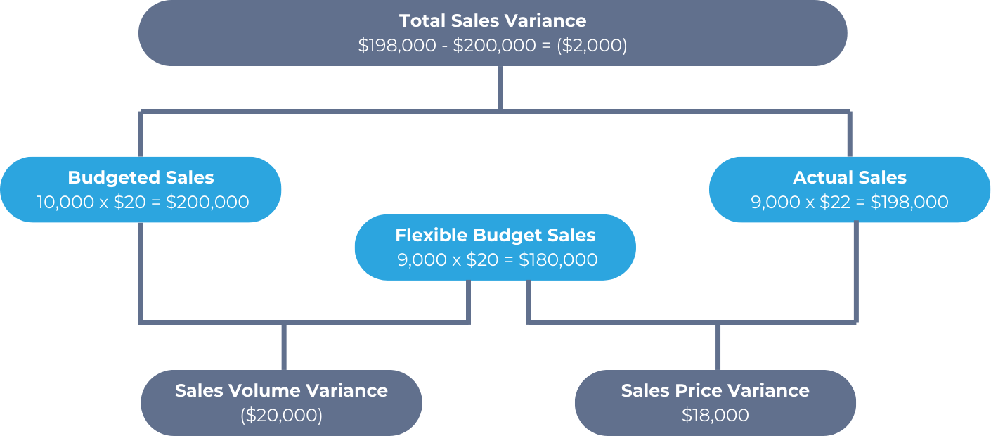
The calculation of the sales variances are further illustrated using the original diagram below:

This comparison highlights that the difference between the master budget and the actual results ($2,000 total sales variance) can be analyzed by splitting it into the sales volume variance and sales price variance. The flexible budget serves as a critical intermediary step in this process.

1.2.1. Sales volume variance

$$\begin{array}{rl}\text{SalesVolume variance}& =\text{Flexible budget sales}-\text{Master budget sales}\\ & =180,000-200,000\\ & =(20,000)\end{array}$$

The unfavorable sales volume variance of $20,000 indicates that selling fewer units than planned resulted in a reduced revenue.

1.2.2. Sales price variance

$$\begin{array}{rl}\text{Sales price variance}& =\text{Actual sales}-\text{Flexible budget sales}\\ & =198,000-180,000\\ & =18,000\end{array}$$

The favorable sales price variance of $18,000 shows that selling products at a higher price offset some of the revenue loss from lower volume.

1.2.3. Total sales variance

$$\begin{array}{rl}\text{Total sales variance}& =\text{Sales volume variance}+\text{Sales price variance}\\ & =(20,000)+18,000\\ & =(2,000)\end{array}$$

Alternatively, the total sales variance can be calculated directly as:

$$\begin{array}{rl}\text{Total sales variance}& =\text{Actual sales}-\text{Master budget sales}\\ & =198,000-200,000\\ & =(2,000)\end{array}$$

This breakdown demonstrates that while pricing strategies were favorable, they did not fully offset the impact of selling fewer units than planned.