The normal distribution

The bell curve discussed in the previous section represents the normal distribution. In a normal distribution, the mean is equal to the median, and the curve is bell-shaped and symmetric.

Empirical Rule (also known as the $68$ - $95$ - $99.7$ rule)

About $68%$ of the data lies within one standard deviation (in either direction) of the mean.
About $95%$ of the data lies within two standard deviations (in either direction) of the mean.
About $99.7%$ of the data (the vast majority) lies within three standard deviations (in either direction) of the mean.

Distributions

A normal distribution also has two inflection points. These are the points where the curve changes concavity (from concave up to concave down, or vice versa). Each inflection point is exactly one standard deviation from the mean. Since the normal distribution is symmetric, the percentages from the empirical rule split evenly on either side of the mean. Each graph below illustrates one level of the rule.

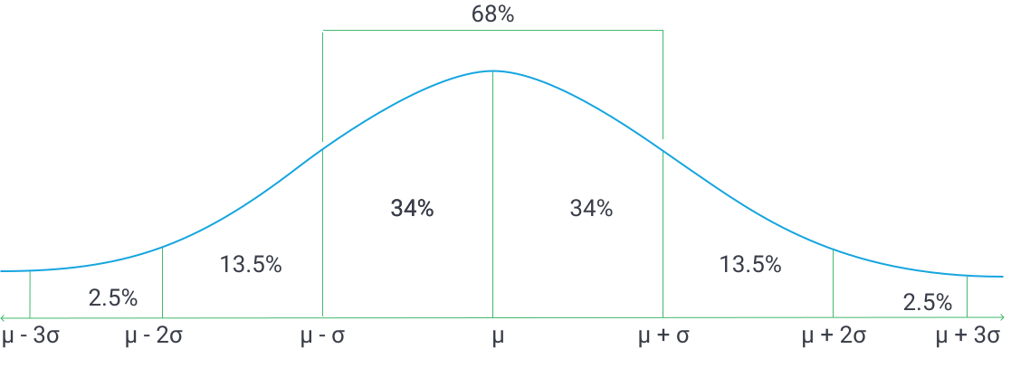
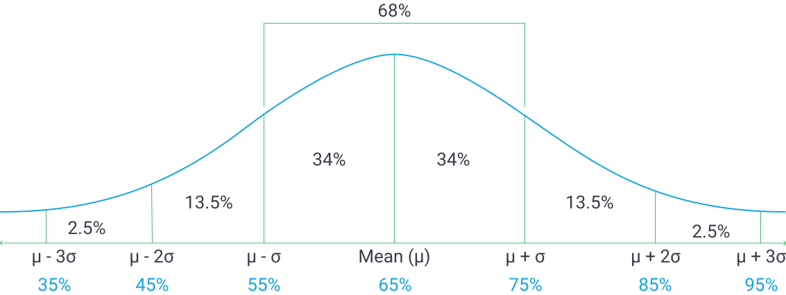
Within 1 standard deviation — $68%$

About $68%$ of the data falls within 1 standard deviation of the mean, which means:

$34%$ falls between the mean and 1 standard deviation above the mean.
$34%$ falls between the mean and 1 standard deviation below the mean.

Bell curve showing data within one standard deviation of the mean. — Normal distribution showing data within one standard deviation

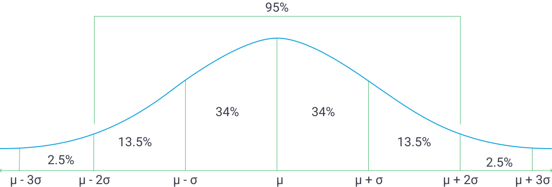
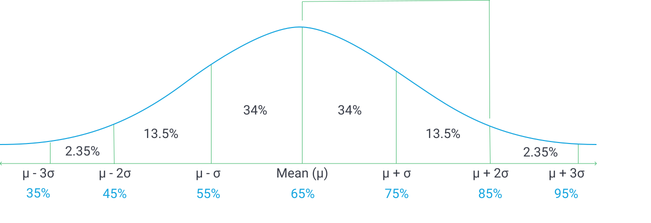
Within 2 standard deviations — $95%$

About $95%$ of the data falls within 2 standard deviations of the mean, which means:

About $13.5%$ falls between 1 and 2 standard deviations below the mean.
About $13.5%$ falls between 1 and 2 standard deviations above the mean.

Bell curve showing data within two standard deviations of the mean. — Normal distribution showing data within two standard deviations

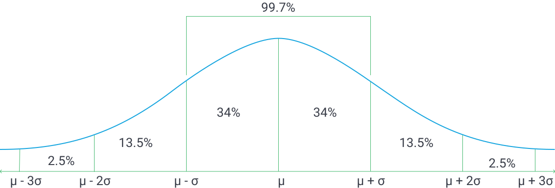
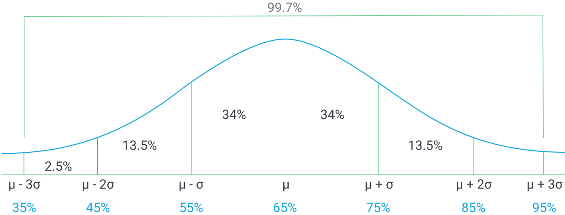
Within 3 standard deviations — $99.7%$

About $99.7%$ of the data falls within 3 standard deviations of the mean, which means:

About $2.35%$ falls between 2 and 3 standard deviations below the mean.
About $2.35%$ falls between 2 and 3 standard deviations above the mean.

Bell curve showing data within three standard deviations of the mean. — Normal distribution showing the 68-95-99.7 rule

Because the normal curve is tightly concentrated around the mean, very few data points fall far out in the tails. In particular, only

0.3%

of the data (about

3

out of every

1000

values) lie more than

3

standard deviations above or below the mean.

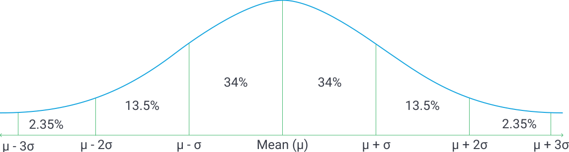
The diagram below shows all three levels together, which is useful for visualizing how the percentages stack across the full distribution.

Bell curve centered at the mean with labeled standard deviations. — Normal distribution intervals

Practice problem

Part a.

The test scores on the Florida standardized math test are normally distributed with a mean of $65%$ and a standard deviation of $10%$ .

a. What percentage of students got a score higher than $65%$ ?

In a normal distribution, the mean and median are equal, so the median is also $65%$ . By definition, half the data lies above the median.

Solution to part a:

(spoiler)

$50%$ of students scored higher than $65%$ .

Part b.

b. What percentage of students scored between $55%$ and $75%$ ?

$55%$ is one standard deviation below the mean: $65% - 10% = 55%$

$75%$ is one standard deviation above the mean: $65% + 10% = 75%$

By the empirical rule, about $68%$ of the data falls within one standard deviation of the mean in either direction.

One standard deviation from the mean

Solution to part b:

(spoiler)

Approximately $68%$ of students scored between $55%$ and $75%$ .

Part c.

c. What percentage of students scored between $65%$ and $85%$ ?

First, identify how far $85%$ is from the mean: $65% + 2 \times 10% = 85%$ , so $85%$ is two standard deviations above the mean.

By the empirical rule, about $95%$ of the data lies within two standard deviations of the mean. Because the normal distribution is symmetric, the area from the mean to two standard deviations above is:

$\frac{95%}{2} = 47.5%$

Mean of 65% with standard deviation

Solution to part c:

(spoiler)

Approximately $47.5%$ of students scored between $65%$ and $85%$ .

Part d.

d. What percentage of students got a score lower than $35%$ ?

First, locate $35%$ relative to the mean: $65% - 3 \times 10% = 35%$ , so $35%$ is three standard deviations below the mean.

From the empirical rule, $99.7%$ of data lies within three standard deviations of the mean, so $0.3%$ lies outside. Because the distribution is symmetric, that $0.3%$ splits evenly between both tails:

$\frac{0.3%}{2} = 0.15%$

Three standard deviations from the mean

Solution to part d:

(spoiler)

Approximately $0.15%$ of students scored lower than $35%$ .

Part e.

e. What percentage of students got a score lower than $75%$ ?

Break the region “below $75%$ ” into two parts:

The percentage at or below the mean ( $65%$ ) is $50%$ , because half the data lies below the mean in a normal distribution.

The percentage between $65%$ and $75%$ is $34%$ , because $75%$ is one standard deviation above the mean and the area from the mean to one standard deviation above is half of $68%$ .

$50% + 34% = 84%$

Three standard deviations from the mean
Solution to part e:

(spoiler)

About $84%$ of students scored lower than $75%$ .

Normal distribution basics

Bell-shaped, symmetric curve
Mean = median = mode
Two inflection points, each 1 standard deviation from mean

Empirical rule (68-95-99.7 rule)

68% of data within 1 standard deviation of mean
95% within 2 standard deviations
99.7% within 3 standard deviations

Distribution of data across standard deviations

68% within ±1 SD:
- 34% between mean and +1 SD
- 34% between mean and -1 SD
95% within ±2 SD:
- 13.5% between +1 and +2 SD
- 13.5% between -1 and -2 SD
99.7% within ±3 SD:
- 2.35% between +2 and +3 SD
- 2.35% between -2 and -3 SD
Only 0.3% beyond ±3 SD (0.15% in each tail)

Key properties

Curve is tightly concentrated around the mean
Tails contain very few data points
Symmetry means percentages split evenly around mean

Example applications

50% above/below mean (median)
68% between 1 SD below and above mean
47.5% between mean and 2 SD above mean
0.15% below 3 SD below mean
84% below 1 SD above mean (mean + 1 SD)

The normal distribution

The bell curve discussed in the previous section represents the normal distribution. In a normal distribution, the mean is equal to the median, and the curve is bell-shaped and symmetric.

Empirical Rule (also known as the $68$ - $95$ - $99.7$ rule)

About $68%$ of the data lies within one standard deviation (in either direction) of the mean.
About $95%$ of the data lies within two standard deviations (in either direction) of the mean.
About $99.7%$ of the data (the vast majority) lies within three standard deviations (in either direction) of the mean.

Distributions

Within 1 standard deviation — $68%$

About $68%$ of the data falls within 1 standard deviation of the mean, which means:

$34%$ falls between the mean and 1 standard deviation above the mean.
$34%$ falls between the mean and 1 standard deviation below the mean.

Within 2 standard deviations — $95%$

About $95%$ of the data falls within 2 standard deviations of the mean, which means:

About $13.5%$ falls between 1 and 2 standard deviations below the mean.
About $13.5%$ falls between 1 and 2 standard deviations above the mean.

Within 3 standard deviations — $99.7%$

About $99.7%$ of the data falls within 3 standard deviations of the mean, which means:

About $2.35%$ falls between 2 and 3 standard deviations below the mean.
About $2.35%$ falls between 2 and 3 standard deviations above the mean.

Because the normal curve is tightly concentrated around the mean, very few data points fall far out in the tails. In particular, only $0.3%$ of the data (about $3$ out of every $1000$ values) lie more than $3$ standard deviations above or below the mean.

The diagram below shows all three levels together, which is useful for visualizing how the percentages stack across the full distribution.

Practice problem

Part a.

The test scores on the Florida standardized math test are normally distributed with a mean of $65%$ and a standard deviation of $10%$ .

a. What percentage of students got a score higher than $65%$ ?

In a normal distribution, the mean and median are equal, so the median is also $65%$ . By definition, half the data lies above the median.

Solution to part a:

(spoiler)

$50%$ of students scored higher than $65%$ .

Part b.

b. What percentage of students scored between $55%$ and $75%$ ?

$55%$ is one standard deviation below the mean: $65% - 10% = 55%$

$75%$ is one standard deviation above the mean: $65% + 10% = 75%$

By the empirical rule, about $68%$ of the data falls within one standard deviation of the mean in either direction.

Solution to part b:

(spoiler)

Approximately $68%$ of students scored between $55%$ and $75%$ .

Part c.

c. What percentage of students scored between $65%$ and $85%$ ?

First, identify how far $85%$ is from the mean: $65% + 2 \times 10% = 85%$ , so $85%$ is two standard deviations above the mean.

By the empirical rule, about $95%$ of the data lies within two standard deviations of the mean. Because the normal distribution is symmetric, the area from the mean to two standard deviations above is:

$\frac{95%}{2} = 47.5%$

Solution to part c:

(spoiler)

Approximately $47.5%$ of students scored between $65%$ and $85%$ .

Part d.

d. What percentage of students got a score lower than $35%$ ?

First, locate $35%$ relative to the mean: $65% - 3 \times 10% = 35%$ , so $35%$ is three standard deviations below the mean.

From the empirical rule, $99.7%$ of data lies within three standard deviations of the mean, so $0.3%$ lies outside. Because the distribution is symmetric, that $0.3%$ splits evenly between both tails:

$\frac{0.3%}{2} = 0.15%$

Solution to part d:

(spoiler)

Approximately $0.15%$ of students scored lower than $35%$ .

Part e.

e. What percentage of students got a score lower than $75%$ ?

Break the region “below $75%$ ” into two parts:

The percentage at or below the mean ( $65%$ ) is $50%$ , because half the data lies below the mean in a normal distribution.

The percentage between $65%$ and $75%$ is $34%$ , because $75%$ is one standard deviation above the mean and the area from the mean to one standard deviation above is half of $68%$ .

$50% + 34% = 84%$

Solution to part e:

(spoiler)

About $84%$ of students scored lower than $75%$ .