


Achievable logoAchievable logo
AP Macroeconomics
Sign in
Sign up
Purchase
Textbook
Practice exams
Support
How it works
Exam catalog
Mountain with a flag at the peak
Textbook
Example
1. Core economic concepts
1.1 First principles
1.2 Opportunity cost examples
1.3 Ricardian trade
1.4 Macroeconomic choice
1.5 Markets
1.6 Demand and supply shifters
2. Measurement of economic performance
3. Modeling of income and prices
4. Financial sector
5. Long-run consequences of stabilization policy
6. Open economy
Achievable logoAchievable logo
1.6 Demand and supply shifters
Achievable AP Macroeconomics
1. Core economic concepts
Our AP Macroeconomics course is currently in development and is a work-in-progress.

Demand and supply shifters

10 min read
Font
Discuss
Share
Feedback

With the concept of equilibrium laid out, we can return to what was set aside in that presentation. Factors other than price that have an impact on either demand or supply.

To frame that we start with a natural question: why are gas prices not exactly the same at every station? Across states it is easy to imagine that each could be considered to be a separate market due to differences in regulations and taxes. But even within a single city, gas prices are often not exactly the same.

What has been presented so far is just a snapshot of a market. The outcome of a single month, day, year, or any specified period of time we are looking at. If nothing changes, then the price and quantity will be the same and the original equilibrium is all that will ever happen. In a more realistic story, changes may not happen every month, but they will happen some months.

For example, in the United States people tend to drive more in the summer than in the winter. Tax incentives for electric cars could lead consumers to buy more of them and therefore need less gas. Gasoline production can be affected by changes in the oil market, as not all oil is exactly identical and refineries are built for processing specific qualities of oil. There are nearly endless possible changes.

How can we assess what happens to a market when those other factors do change? That is our next topic.

Demand shifters

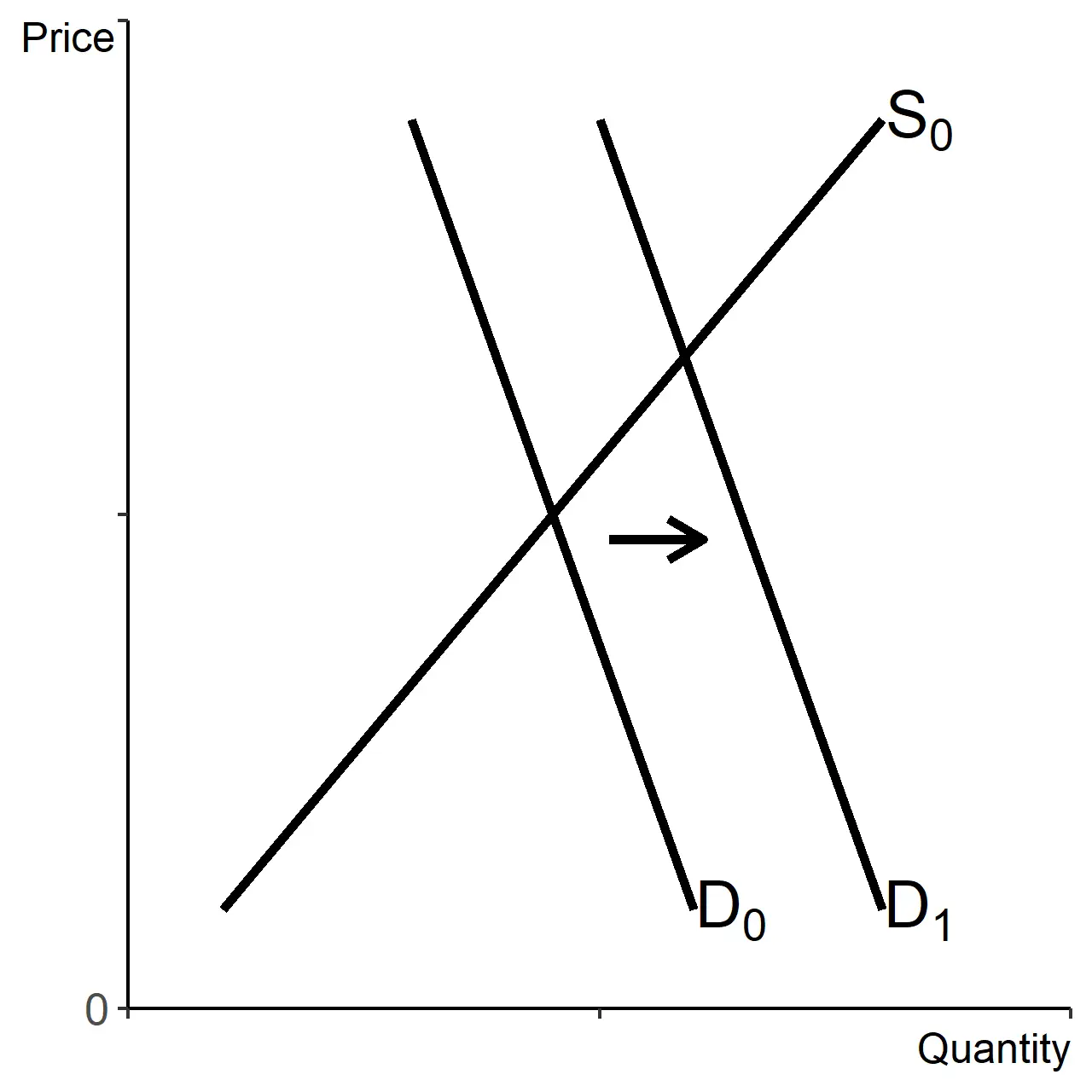
Demand curve shifts to the right (or up).
An increase in demand

If any non-price factor changes, that breaks our ceteris paribus assumption. We refer to such things as shifters.

We can categorize demand shifters, using the acronym TIMER.

  • T - tastes and preferences
  • I - income
  • M - market size
  • E - expectations about future prices
  • R - related goods (prices of them)

An increase in demand is equal to the quantity demanded being higher for every price, holding all other factors equal. This is a shift right of the demand curve. It can also be described as a shift up. It is helpful to remember that for all curves, when we say it increases or decreases, we are always referring to what happens to the quantity.

The following table summarizes how changes in our factors impact demand. The second column describes what change would shift demand to the right. The third column describes what change would shift demand to the left. It will always be the case that switching the direction of a change, from positive to negative or negative to positive, simply switches the resulting shift in demand.

Factor D→ / ↑ D← / ↓
Tastes and preferences Increase Decrease
Income Increase Decrease
Market size Increase Decrease
Expectations about future prices Increase Decrease
Price for goods used together Decrease Increase
Price for goods we choose between Increase Decrease

Before we talked about trips to the store and driving for fun as uses that can increase when prices fall. It may just be that some people live in a city and love nature and so they always drive further on the weekend. Someone else may love video games, so they never leave their house on the weekend. This is what we mean by tastes and preferences. Something like improved weather leading to more driving overall would also qualify as an increase due to tastes and preferences.

Income and market size are uncomplicated. If either one is larger, that leads to an increase in demand. So for every price, the quantity demanded increases if income or market size is higher and decreases if income or market size is lower.

Expectations about future prices have an effect because consumers desire to spend less, all else equal. If consumers expect higher prices tomorrow, that increases demand today when the good is relatively cheaper. If they expect lower prices they will prefer to wait and that decreases demand today.

Related goods are just a little more complicated. We have goods that are used together, such as chips and salsa, and goods that people choose between, such as coffee and tea.

For goods that are used together, a fall in the price of one makes demand for the other rise. If the price of salsa falls, demand for chips increases. Similarly, if the price of chips falls, then demand for salsa increases. In this case the price of another good is negatively related to demand.

Unsurprisingly, goods that people choose between have the opposite relationship. For goods that consumers choose between, the price of one is positively related to demand for the other. If the price of coffee rises, some consumers will switch and buy tea instead. This increases the demand for tea. Similarly, if the price of tea falls, some consumers will switch and buy tea instead of coffee. This makes demand for coffee fall.

Supply shifters

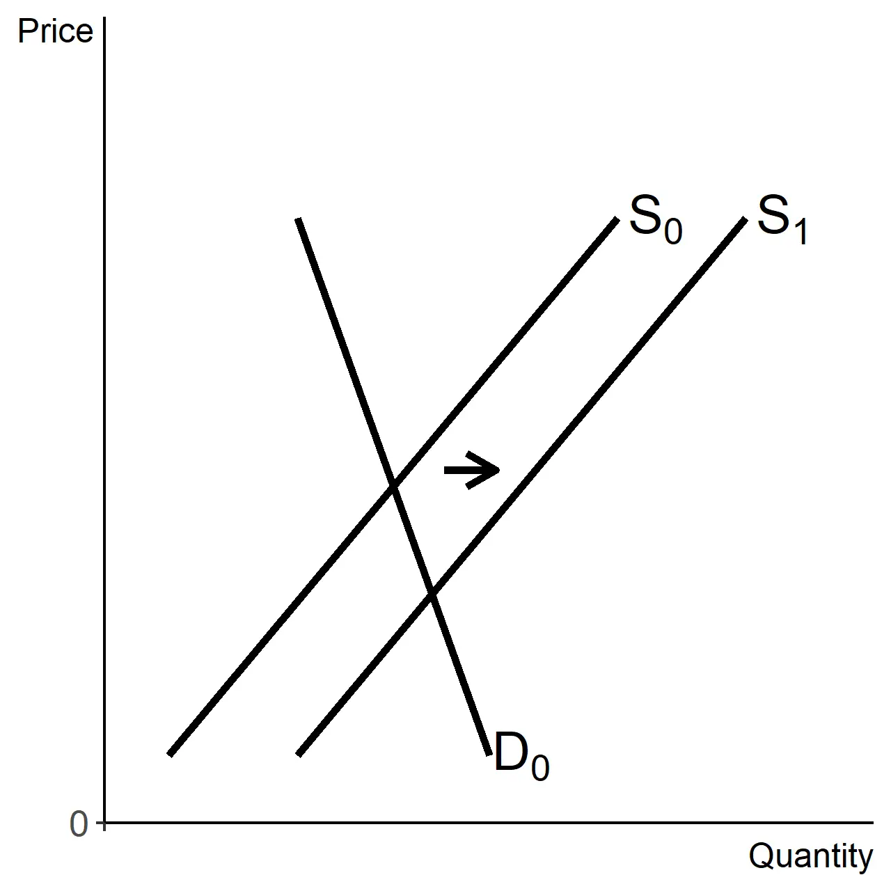
Supply curve shifts to the right (or down).
An increase in supply

To keep in mind the shifters of supply, the suggested acronym is TINGE.

  • T - technology and productivity
  • I - input prices
  • N - number of producers
  • G - government policies
  • E - expectations of future prices

Just as with demand, we start with a table that summarizes these factors and what changes in them lead to increases and decreases in supply.

Factor S→ / ↓ S← / ↑
Technology and productivity Decrease Increase
Input prices Increase Decrease
Number of producers Decrease Increase
Government policies
Taxes and regulations Increase Decrease
Subsidies Decrease Increase
Expectations about future prices Increase Decrease

First is technology and productivity. Any development that makes production quicker or enables a lower cost for the same speed, shifts the supply curve to the right (down). Input prices follow a similar logic. If they fall, that lowers costs for firms.

The number of producers has to do with market forces rather than specific firm costs. For any situation with many sellers, more firms leads to a higher quantity supplied for every price and fewer firms leads to a lower quantity supplied for every price.

Government policies can hit on any of the previous stories. Taxes will generally make costs higher, subsidies will make costs lower. Subsidies will generally increase the number of producers and taxes will reduce the number of producers. Regulations will generally be thought of similarly, with more regulations lowering the number of firms and increasing costs and the removal of regulations increasing the number of firms and decreasing costs.

As a general rule anything that lower costs for producing firms is always associated with a rightward shift of the supply curve. This is equivalent to a lower price for each quantity supplied.

Finally, we have expectations of future prices. The logic here is exactly the opposite of what occurs with the demand curve. If producers expect higher prices in the future, they want to sell less today, since future sales will lead to more revenue.

Equilibrium changes

Following shifts in demand or supply, often what we are most interested in is the impact to the equilibrium quantity and price. Here when we use all else equal, what we mean is that the story behind our shift is the only change in the market. Thus we deal with one shift at a time.

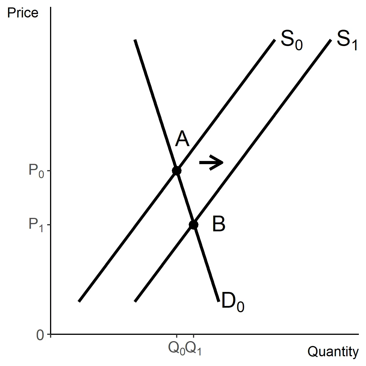
When looking at a complete market, a shift in supply can also be described as moving along a single demand curve. Viewed that way, it can be seen that any factor that increases supply will lead to a higher equilibrium price and lower equilibrium quantity. Reversing the story, a decrease in supply leads to a lower price and higher quantity in equilibrium.

Rightward shift of the supply curve, lower P and higher Q.
Supply shift

The graph above shows an increase in supply, which moves the equilibrium from point A to point B. Described another way, it decreases the equilibrium price from P0​ to P1​ and increases the equilibrium quantity from Q0​ to Q1​.

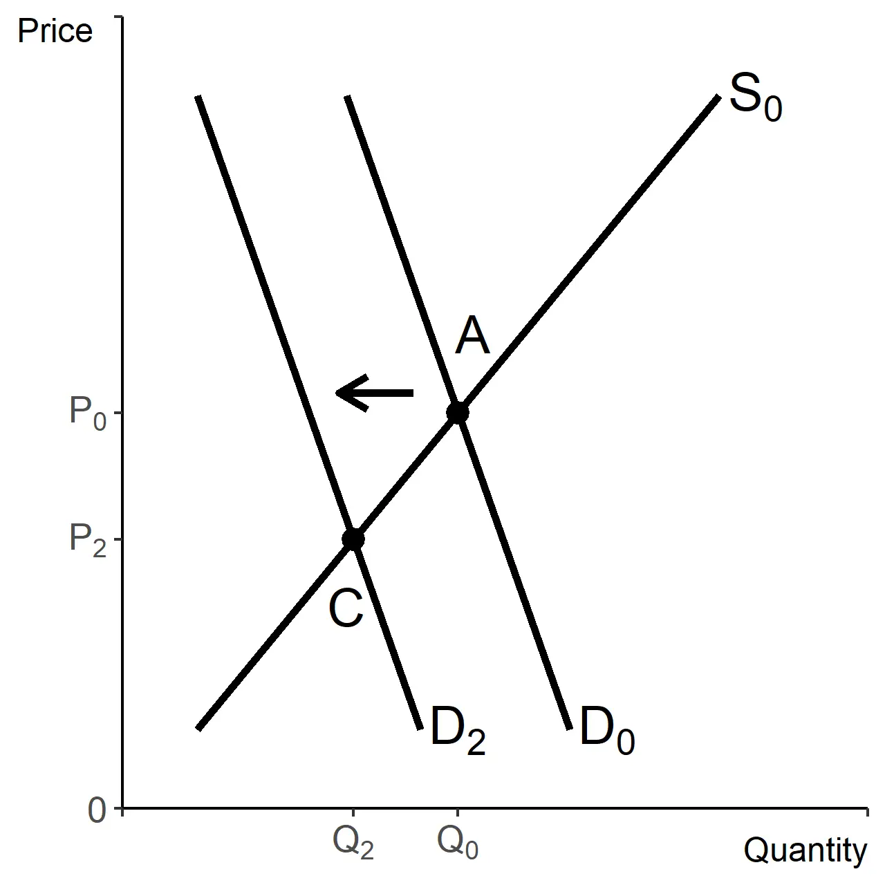
Switching from supply shifts to demand shifts leads to a similar relationship. Demand shifts are equivalent to movements along a single supply curve. Any factor that decreases demand (shifts supply left) will lead to a higher equilibrium price and a lower equilibrium quantity.

Leftward shift of the demand curve, lower P and lower Q.
Demand shift

The graph above shows a decrease in demand, which moves the equilibrium from point A to point C. More specifically, it decreases the equilibrium price from P0​ to P2​ and decreases the equilibrium quantity from Q0​ to Q2​.

Whenever we make any sort of adjustment, we will assume that that is the only change in our market and most commonly it will only affect one side of our market. It is rare to see multiple changes at the same time that cause opposing effects to the same curve, because then the outcome depends on which curve moves more.

This table summarizes the results of various shift combinations. Note that when both curves shift, one change is clear and the other is ambiguous.

Shift or shifts Change in P Change in Q
D increase Higher Lower
D decrease Lower Higher
S increase Lower Higher
S decrease Higher Lower
S and D increase Unknown Higher
S and D decrease Unknown Lower
S increase, D decrease Lower Unknown
D increase, S decrease Higher Unknown

Multiple shifts can take place in sequence. For example a FRQ may set up a market in part (a). Then part (b) adds a shift and ask for an assessment of the new change. Part © may either go back to (a) and introduce a different shift or add another shift on top of part (b).

To close, these shifts and stories have been describing a single market. Such as the market for gasoline. Other examples could be cars, fruit, smartphones. We will have many macroeconomic markets that follow this structure, such as the markets for loanable funds and foreign exchange.

Later we will expand this to a model of the entire economy. That will be aggregate supply and aggregate demand, but which will have its own special shifts and relationships.

Demand shifters (TIMER)

  • Tastes and preferences: changes shift demand curve
  • Income and market size: higher values increase demand at every price
  • Expectations of future prices: expected price rises increase current demand
  • Related goods:
    • Complements: price drop in one increases demand for the other
    • Substitutes: price rise in one increases demand for the other

Supply shifters (TINGE)

  • Technology and productivity: improvements shift supply right (increase)
  • Input prices: lower input costs increase supply
  • Number of producers: more producers increase supply
  • Government policies: taxes decrease, subsidies increase supply
  • Expectations of future prices: expected price rise decreases current supply

Equilibrium changes

  • Supply increase: lower equilibrium price, higher equilibrium quantity
  • Demand increase: higher equilibrium price, higher equilibrium quantity
  • Multiple shifts: analyze sequentially, not simultaneously with opposing effects
  • Changes apply to any single market (e.g., gasoline, cars, fruit)
Previous
Next  | 2.1 Circular flow model
All rights reserved ©2016 - 2026 Achievable, Inc.

Demand and supply shifters

With the concept of equilibrium laid out, we can return to what was set aside in that presentation. Factors other than price that have an impact on either demand or supply.

To frame that we start with a natural question: why are gas prices not exactly the same at every station? Across states it is easy to imagine that each could be considered to be a separate market due to differences in regulations and taxes. But even within a single city, gas prices are often not exactly the same.

What has been presented so far is just a snapshot of a market. The outcome of a single month, day, year, or any specified period of time we are looking at. If nothing changes, then the price and quantity will be the same and the original equilibrium is all that will ever happen. In a more realistic story, changes may not happen every month, but they will happen some months.

For example, in the United States people tend to drive more in the summer than in the winter. Tax incentives for electric cars could lead consumers to buy more of them and therefore need less gas. Gasoline production can be affected by changes in the oil market, as not all oil is exactly identical and refineries are built for processing specific qualities of oil. There are nearly endless possible changes.

How can we assess what happens to a market when those other factors do change? That is our next topic.

Demand shifters

If any non-price factor changes, that breaks our ceteris paribus assumption. We refer to such things as shifters.

We can categorize demand shifters, using the acronym TIMER.

  • T - tastes and preferences
  • I - income
  • M - market size
  • E - expectations about future prices
  • R - related goods (prices of them)

An increase in demand is equal to the quantity demanded being higher for every price, holding all other factors equal. This is a shift right of the demand curve. It can also be described as a shift up. It is helpful to remember that for all curves, when we say it increases or decreases, we are always referring to what happens to the quantity.

The following table summarizes how changes in our factors impact demand. The second column describes what change would shift demand to the right. The third column describes what change would shift demand to the left. It will always be the case that switching the direction of a change, from positive to negative or negative to positive, simply switches the resulting shift in demand.

Factor D→ / ↑ D← / ↓
Tastes and preferences Increase Decrease
Income Increase Decrease
Market size Increase Decrease
Expectations about future prices Increase Decrease
Price for goods used together Decrease Increase
Price for goods we choose between Increase Decrease

Before we talked about trips to the store and driving for fun as uses that can increase when prices fall. It may just be that some people live in a city and love nature and so they always drive further on the weekend. Someone else may love video games, so they never leave their house on the weekend. This is what we mean by tastes and preferences. Something like improved weather leading to more driving overall would also qualify as an increase due to tastes and preferences.

Income and market size are uncomplicated. If either one is larger, that leads to an increase in demand. So for every price, the quantity demanded increases if income or market size is higher and decreases if income or market size is lower.

Expectations about future prices have an effect because consumers desire to spend less, all else equal. If consumers expect higher prices tomorrow, that increases demand today when the good is relatively cheaper. If they expect lower prices they will prefer to wait and that decreases demand today.

Related goods are just a little more complicated. We have goods that are used together, such as chips and salsa, and goods that people choose between, such as coffee and tea.

For goods that are used together, a fall in the price of one makes demand for the other rise. If the price of salsa falls, demand for chips increases. Similarly, if the price of chips falls, then demand for salsa increases. In this case the price of another good is negatively related to demand.

Unsurprisingly, goods that people choose between have the opposite relationship. For goods that consumers choose between, the price of one is positively related to demand for the other. If the price of coffee rises, some consumers will switch and buy tea instead. This increases the demand for tea. Similarly, if the price of tea falls, some consumers will switch and buy tea instead of coffee. This makes demand for coffee fall.

Supply shifters

To keep in mind the shifters of supply, the suggested acronym is TINGE.

  • T - technology and productivity
  • I - input prices
  • N - number of producers
  • G - government policies
  • E - expectations of future prices

Just as with demand, we start with a table that summarizes these factors and what changes in them lead to increases and decreases in supply.

Factor S→ / ↓ S← / ↑
Technology and productivity Decrease Increase
Input prices Increase Decrease
Number of producers Decrease Increase
Government policies
Taxes and regulations Increase Decrease
Subsidies Decrease Increase
Expectations about future prices Increase Decrease

First is technology and productivity. Any development that makes production quicker or enables a lower cost for the same speed, shifts the supply curve to the right (down). Input prices follow a similar logic. If they fall, that lowers costs for firms.

The number of producers has to do with market forces rather than specific firm costs. For any situation with many sellers, more firms leads to a higher quantity supplied for every price and fewer firms leads to a lower quantity supplied for every price.

Government policies can hit on any of the previous stories. Taxes will generally make costs higher, subsidies will make costs lower. Subsidies will generally increase the number of producers and taxes will reduce the number of producers. Regulations will generally be thought of similarly, with more regulations lowering the number of firms and increasing costs and the removal of regulations increasing the number of firms and decreasing costs.

As a general rule anything that lower costs for producing firms is always associated with a rightward shift of the supply curve. This is equivalent to a lower price for each quantity supplied.

Finally, we have expectations of future prices. The logic here is exactly the opposite of what occurs with the demand curve. If producers expect higher prices in the future, they want to sell less today, since future sales will lead to more revenue.

Equilibrium changes

Following shifts in demand or supply, often what we are most interested in is the impact to the equilibrium quantity and price. Here when we use all else equal, what we mean is that the story behind our shift is the only change in the market. Thus we deal with one shift at a time.

When looking at a complete market, a shift in supply can also be described as moving along a single demand curve. Viewed that way, it can be seen that any factor that increases supply will lead to a higher equilibrium price and lower equilibrium quantity. Reversing the story, a decrease in supply leads to a lower price and higher quantity in equilibrium.

The graph above shows an increase in supply, which moves the equilibrium from point A to point B. Described another way, it decreases the equilibrium price from P0​ to P1​ and increases the equilibrium quantity from Q0​ to Q1​.

Switching from supply shifts to demand shifts leads to a similar relationship. Demand shifts are equivalent to movements along a single supply curve. Any factor that decreases demand (shifts supply left) will lead to a higher equilibrium price and a lower equilibrium quantity.

The graph above shows a decrease in demand, which moves the equilibrium from point A to point C. More specifically, it decreases the equilibrium price from P0​ to P2​ and decreases the equilibrium quantity from Q0​ to Q2​.

Whenever we make any sort of adjustment, we will assume that that is the only change in our market and most commonly it will only affect one side of our market. It is rare to see multiple changes at the same time that cause opposing effects to the same curve, because then the outcome depends on which curve moves more.

This table summarizes the results of various shift combinations. Note that when both curves shift, one change is clear and the other is ambiguous.

Shift or shifts Change in P Change in Q
D increase Higher Lower
D decrease Lower Higher
S increase Lower Higher
S decrease Higher Lower
S and D increase Unknown Higher
S and D decrease Unknown Lower
S increase, D decrease Lower Unknown
D increase, S decrease Higher Unknown

Multiple shifts can take place in sequence. For example a FRQ may set up a market in part (a). Then part (b) adds a shift and ask for an assessment of the new change. Part © may either go back to (a) and introduce a different shift or add another shift on top of part (b).

To close, these shifts and stories have been describing a single market. Such as the market for gasoline. Other examples could be cars, fruit, smartphones. We will have many macroeconomic markets that follow this structure, such as the markets for loanable funds and foreign exchange.

Later we will expand this to a model of the entire economy. That will be aggregate supply and aggregate demand, but which will have its own special shifts and relationships.

Key points

Demand shifters (TIMER)

  • Tastes and preferences: changes shift demand curve
  • Income and market size: higher values increase demand at every price
  • Expectations of future prices: expected price rises increase current demand
  • Related goods:
    • Complements: price drop in one increases demand for the other
    • Substitutes: price rise in one increases demand for the other

Supply shifters (TINGE)

  • Technology and productivity: improvements shift supply right (increase)
  • Input prices: lower input costs increase supply
  • Number of producers: more producers increase supply
  • Government policies: taxes decrease, subsidies increase supply
  • Expectations of future prices: expected price rise decreases current supply

Equilibrium changes

  • Supply increase: lower equilibrium price, higher equilibrium quantity
  • Demand increase: higher equilibrium price, higher equilibrium quantity
  • Multiple shifts: analyze sequentially, not simultaneously with opposing effects
  • Changes apply to any single market (e.g., gasoline, cars, fruit)

More from Core economic concepts

  • First principles
  • Opportunity cost examples
  • Ricardian trade
  • Macroeconomic choice
  • Markets