


Achievable logoAchievable logo
AP Macroeconomics
Sign in
Sign up
Purchase
Textbook
Practice exams
Support
How it works
Exam catalog
Mountain with a flag at the peak
Textbook
Example
1. Core economic concepts
1.1 First principles
1.2 Opportunity cost examples
1.3 Ricardian trade
1.4 Macroeconomic choice
1.5 Markets
1.6 Demand and supply shifters
2. Measurement of economic performance
3. Modeling of income and prices
4. Financial sector
5. Long-run consequences of stabilization policy
6. Open economy
Achievable logoAchievable logo
1.2 Opportunity cost examples
Achievable AP Macroeconomics
1. Core economic concepts
Our AP Macroeconomics course is currently in development and is a work-in-progress.

Opportunity cost examples

9 min read
Font
Discuss
Share
Feedback

Opportunity cost is our first concept so important that we need to look at some extended examples to illustrate it. This subchapter starts with a couple of examples involving personal trade-offs, before turning to an important macroeconomic take on opportunity cost - the production possibilities curve.

Budget example

A simple example we can start with is the choice of what to buy when going out for fast food. To keep things simple let us go back to McDonald’s in 1955. Assume that we have 35 cents to spend and our our options are:

  • Hamburger (15 cents)
  • French fries (10 cents)
  • Milkshake (20 cents)

Ignoring tax, there are a number of combinations that we could afford. Two possibilities where we spend all 35 cents are that we could get a hamburger and a milkshake (15+20=35) or a hamburger and two french fries (15+2×10=35).

We could also buy a hamburger and french fry and have 10 cents leftover (15+10=25). In economics we will generally focus on examples where there is nothing left over, but in real-life decisions that is often something that happens because an individual decision is just one piece of a bigger picture.

In this McDonald’s example, we can see that one milkshake and two french fries have the same cost. So the opportunity cost of one milkshake can be viewed as two orders of french fries, or one french fry being equal to half of a milkshake.

In our next subchapter we will cover trade-offs involving production, thinking about how to allocate time to produce two goods. While we will be able to (and want to) discuss the trade-off between units of the goods directly, the root of those types of trade-offs will be that each good is produced using the same resource (labor).

College versus work

A deeper example is the choice of going to college. Each year of school has various measures of cost, and this presents an opportunity to clarify the difference between net and gross. A gross value is the dollar amount without any adjustments. Conceptually, it is a sticker price, in this case the prices of tuition, fees, and room and board.

Net values, on the other hand, reflect what is paid out of pocket. So the net is the gross, adjusted for things such as discounts, rebates, or added fees. If added fees sound strange, consider one you may have seen in real life. Some stores and restaurants charge an extra percentage for using a credit card. So the net cost can be different depending on how we choose to pay.

For our tuition example, the net cost includes all gross costs, tuition, fees, and room and board, with amounts of financial aid and scholarships taken out. Thus net values are what we really need, but they will usually not be opportunity cost on their own. The full opportunity cost must also account for that value of our next best choice.

For each year we not only have to pay for school, but we also give up earning wages. The basic trade-off is that we pay now and miss out on earning, in exchange for higher wages once we graduate. To compare we will want to calculate net lifetime earnings to see which option pays better.

To be realistic, there are other factors to add. Not every school has the same costs, not every major has the same earnings, and earnings and costs are not likely to be constant each year. Importantly, a dollar today and a dollar in future years are not worth the same. If we make educated guesses, we can calculate, but changing these guesses can change our decision.

##The production possibilities curve Models will be a critical component of our study of macroeconomics and another of the “Big Ideas” that will appear throughout the course. They are simplified descriptions of behavior, making assumptions to cut down on the details we have to consider in order to say something meaningful about an economic question.

The production possibilities curve (or PPC) is our first model of the macroeconomy. We start by setting up our assumptions for our sample country.

  • There are two goods that can be produced: food or microchips
  • There are no prices, but trade-offs exist
  • There is a fixed trade-off in production, we can costlessly switch from one good to the other
  • There is no trade, we sometimes call this autarky

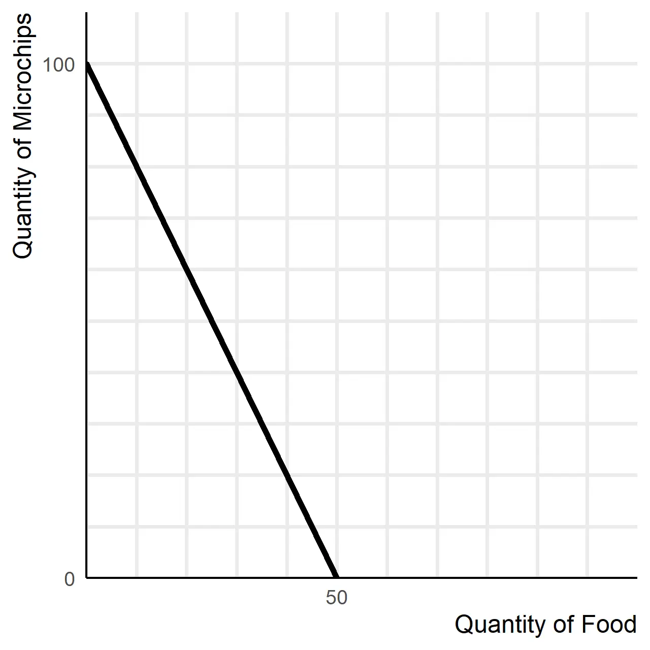
This leads to the graph below, which shows the production possibilities curve. Even though we are labeling this a “curve” in AP Macroeconomics most examples presented with numbers will be linear.

Linear PPF: 100 microchips or 50 units of food
Production possibilities frontier (PPF)

The curve represents the set of maximum combinations of each good we can produce at the same time. Anything inside the curve, including the curve itself, is feasible, or within our capacity to produce. All points outside of the curve are infeasible, or not possible for us to produce.

The numbers presented in this graph give us a lot of important information. The value on the x-axis tells us how many units of food we can produce if our country only makes food, 20 billion units. The value on the y-axis tells us how many units of microchips we can produce if we only make microchips, 100 billion units. Every other point on the graph gives a combination of food and microchips that we can make with the resources we have available to produce.

The absolute value of the slope of the PPC gives us the opportunity cost of microchips in terms of food, ​−10020​​=0.2. In general, that opportunity cost is what we gain of the x-axis good for giving up one unit of the y-axis good as well as what we have to give up of the x-axis good to gain one additional unit of the y-axis good. What we give up can always be viewed as a cost, and what is gained can be viewed as a benefit, as long as we keep in mind that these are in terms of physical units of goods and not money.

Every time we give up one unit of microchips we gain 10020​=0.2 units of food. And to gain one unit of microchips we would have to give up 0.2 units of food. For this example have forced it to be constant, so there is a fixed trade off in production. This means that every unit “costs” the same, so to produce 10 additional units of microchips we would need to give up 10×0.2=2 units of food. Only when the PPC is linear can we use this simplification.

And similarly every time we give up one unit of food, we gain 20100​=5 units of microchips. This type of analysis can always be viewed moving in each direction along the curve.

It is possible to use PPCs for more than just countries. We could use regions, states, cities or even individual factories or workshops. Efficiency For most of our discussions, efficiency is our concept of achieving the optimal or most desirable outcome.

Definitions
Efficiency
The optimal use of scarce resources to produce goods and services

Efficiency is often about maximizing net benefits or minimizing waste. As a starting point efficiency can be thought of as allocating all available resources when we have a decision to make. Something that will get much attention is household decisions, and in macroeconomics all available income can be split into consumption and savings. Consumption will be anything we spend in a year, on any good or service. Savings is most simply everything that we do not spend, which will be a bit broader than savings in a personal finance sense. Thus “spending” need not represent use immediately, just that goods and services are paid for.

Efficiency is a fairly general term. So we add two more specific definitions of efficiency that are relevant for our macroeconomic stories.

Definitions
Productive efficiency
When production occurs at the lowest possible cost.
Allocative efficiency
When production represents society’s preferences.

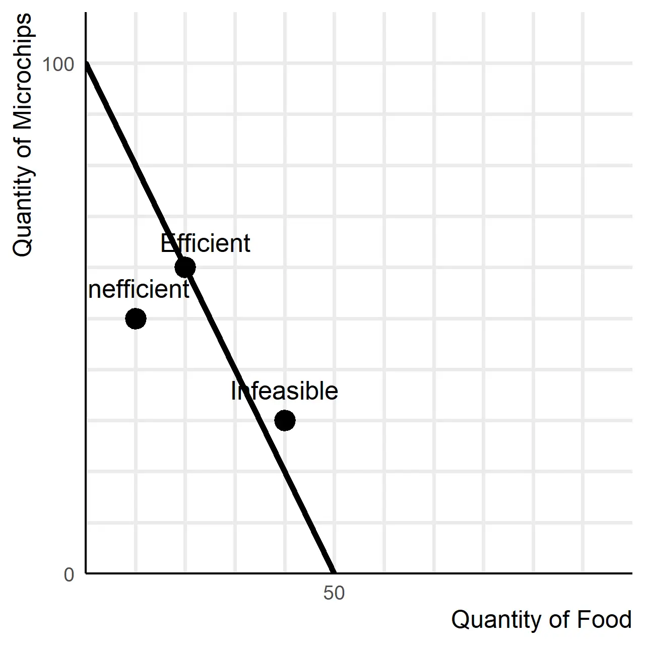
In terms of the PPC, productive efficiency simply requires using all of the resources available. This allows us to split the set of feasible points into efficient and inefficient points. Every combination along the curve itself is productively efficient, while every value inside of the curve is inefficient. That is because if we are ever producing inside of the curve, it is possible for us to gain more production with more effective utilization of our resources.

Examples of this categorization of different allocations are shown in the image below.

Efficient point on curve, inefficient point inside, infeasible point outside
Categories of all

At least for the PPC, allocative efficiency is generally not shown at this level. We may be told that a point represents the ideal production for society, but if that is not given to us we simply cannot say anything at all.

Opportunity cost: key concept

  • Value of next best alternative forgone
  • Illustrated through personal and macroeconomic trade-offs

Budget example

  • Trade-offs in spending limited resources (e.g., 35 cents at McDonald’s)
  • Opportunity cost: what is given up to obtain something else
    • E.g., 1 milkshake = 2 orders of french fries

College versus work

  • Gross value: total cost before adjustments (tuition, fees, room & board)
  • Net value: actual out-of-pocket cost (gross minus aid/scholarships)
  • Full opportunity cost: net cost of college plus forgone wages
    • Compare net lifetime earnings for decision-making

Production possibilities curve (PPC)

  • Model showing maximum combinations of two goods producible with fixed resources
  • Points on/inside curve: feasible; outside: infeasible
  • Slope of PPC = opportunity cost of one good in terms of the other
    • E.g., |−20/100| = 0.2 units of food per microchip
  • Linear PPC: constant opportunity cost; non-linear: opportunity cost varies
  • Moving along curve illustrates trade-offs and opportunity costs in production

Sign up for free to take 4 quiz questions on this topic

Previous
Next  | 1.3 Ricardian trade
All rights reserved ©2016 - 2026 Achievable, Inc.

Opportunity cost examples

Opportunity cost is our first concept so important that we need to look at some extended examples to illustrate it. This subchapter starts with a couple of examples involving personal trade-offs, before turning to an important macroeconomic take on opportunity cost - the production possibilities curve.

Budget example

A simple example we can start with is the choice of what to buy when going out for fast food. To keep things simple let us go back to McDonald’s in 1955. Assume that we have 35 cents to spend and our our options are:

  • Hamburger (15 cents)
  • French fries (10 cents)
  • Milkshake (20 cents)

Ignoring tax, there are a number of combinations that we could afford. Two possibilities where we spend all 35 cents are that we could get a hamburger and a milkshake (15+20=35) or a hamburger and two french fries (15+2×10=35).

We could also buy a hamburger and french fry and have 10 cents leftover (15+10=25). In economics we will generally focus on examples where there is nothing left over, but in real-life decisions that is often something that happens because an individual decision is just one piece of a bigger picture.

In this McDonald’s example, we can see that one milkshake and two french fries have the same cost. So the opportunity cost of one milkshake can be viewed as two orders of french fries, or one french fry being equal to half of a milkshake.

In our next subchapter we will cover trade-offs involving production, thinking about how to allocate time to produce two goods. While we will be able to (and want to) discuss the trade-off between units of the goods directly, the root of those types of trade-offs will be that each good is produced using the same resource (labor).

College versus work

A deeper example is the choice of going to college. Each year of school has various measures of cost, and this presents an opportunity to clarify the difference between net and gross. A gross value is the dollar amount without any adjustments. Conceptually, it is a sticker price, in this case the prices of tuition, fees, and room and board.

Net values, on the other hand, reflect what is paid out of pocket. So the net is the gross, adjusted for things such as discounts, rebates, or added fees. If added fees sound strange, consider one you may have seen in real life. Some stores and restaurants charge an extra percentage for using a credit card. So the net cost can be different depending on how we choose to pay.

For our tuition example, the net cost includes all gross costs, tuition, fees, and room and board, with amounts of financial aid and scholarships taken out. Thus net values are what we really need, but they will usually not be opportunity cost on their own. The full opportunity cost must also account for that value of our next best choice.

For each year we not only have to pay for school, but we also give up earning wages. The basic trade-off is that we pay now and miss out on earning, in exchange for higher wages once we graduate. To compare we will want to calculate net lifetime earnings to see which option pays better.

To be realistic, there are other factors to add. Not every school has the same costs, not every major has the same earnings, and earnings and costs are not likely to be constant each year. Importantly, a dollar today and a dollar in future years are not worth the same. If we make educated guesses, we can calculate, but changing these guesses can change our decision.

##The production possibilities curve Models will be a critical component of our study of macroeconomics and another of the “Big Ideas” that will appear throughout the course. They are simplified descriptions of behavior, making assumptions to cut down on the details we have to consider in order to say something meaningful about an economic question.

The production possibilities curve (or PPC) is our first model of the macroeconomy. We start by setting up our assumptions for our sample country.

  • There are two goods that can be produced: food or microchips
  • There are no prices, but trade-offs exist
  • There is a fixed trade-off in production, we can costlessly switch from one good to the other
  • There is no trade, we sometimes call this autarky

This leads to the graph below, which shows the production possibilities curve. Even though we are labeling this a “curve” in AP Macroeconomics most examples presented with numbers will be linear.

The curve represents the set of maximum combinations of each good we can produce at the same time. Anything inside the curve, including the curve itself, is feasible, or within our capacity to produce. All points outside of the curve are infeasible, or not possible for us to produce.

The numbers presented in this graph give us a lot of important information. The value on the x-axis tells us how many units of food we can produce if our country only makes food, 20 billion units. The value on the y-axis tells us how many units of microchips we can produce if we only make microchips, 100 billion units. Every other point on the graph gives a combination of food and microchips that we can make with the resources we have available to produce.

The absolute value of the slope of the PPC gives us the opportunity cost of microchips in terms of food, ​−10020​​=0.2. In general, that opportunity cost is what we gain of the x-axis good for giving up one unit of the y-axis good as well as what we have to give up of the x-axis good to gain one additional unit of the y-axis good. What we give up can always be viewed as a cost, and what is gained can be viewed as a benefit, as long as we keep in mind that these are in terms of physical units of goods and not money.

Every time we give up one unit of microchips we gain 10020​=0.2 units of food. And to gain one unit of microchips we would have to give up 0.2 units of food. For this example have forced it to be constant, so there is a fixed trade off in production. This means that every unit “costs” the same, so to produce 10 additional units of microchips we would need to give up 10×0.2=2 units of food. Only when the PPC is linear can we use this simplification.

And similarly every time we give up one unit of food, we gain 20100​=5 units of microchips. This type of analysis can always be viewed moving in each direction along the curve.

It is possible to use PPCs for more than just countries. We could use regions, states, cities or even individual factories or workshops. Efficiency For most of our discussions, efficiency is our concept of achieving the optimal or most desirable outcome.

Definitions
Efficiency
The optimal use of scarce resources to produce goods and services

Efficiency is often about maximizing net benefits or minimizing waste. As a starting point efficiency can be thought of as allocating all available resources when we have a decision to make. Something that will get much attention is household decisions, and in macroeconomics all available income can be split into consumption and savings. Consumption will be anything we spend in a year, on any good or service. Savings is most simply everything that we do not spend, which will be a bit broader than savings in a personal finance sense. Thus “spending” need not represent use immediately, just that goods and services are paid for.

Efficiency is a fairly general term. So we add two more specific definitions of efficiency that are relevant for our macroeconomic stories.

Definitions
Productive efficiency
When production occurs at the lowest possible cost.
Allocative efficiency
When production represents society’s preferences.

In terms of the PPC, productive efficiency simply requires using all of the resources available. This allows us to split the set of feasible points into efficient and inefficient points. Every combination along the curve itself is productively efficient, while every value inside of the curve is inefficient. That is because if we are ever producing inside of the curve, it is possible for us to gain more production with more effective utilization of our resources.

Examples of this categorization of different allocations are shown in the image below.

At least for the PPC, allocative efficiency is generally not shown at this level. We may be told that a point represents the ideal production for society, but if that is not given to us we simply cannot say anything at all.

Key points

Opportunity cost: key concept

  • Value of next best alternative forgone
  • Illustrated through personal and macroeconomic trade-offs

Budget example

  • Trade-offs in spending limited resources (e.g., 35 cents at McDonald’s)
  • Opportunity cost: what is given up to obtain something else
    • E.g., 1 milkshake = 2 orders of french fries

College versus work

  • Gross value: total cost before adjustments (tuition, fees, room & board)
  • Net value: actual out-of-pocket cost (gross minus aid/scholarships)
  • Full opportunity cost: net cost of college plus forgone wages
    • Compare net lifetime earnings for decision-making

Production possibilities curve (PPC)

  • Model showing maximum combinations of two goods producible with fixed resources
  • Points on/inside curve: feasible; outside: infeasible
  • Slope of PPC = opportunity cost of one good in terms of the other
    • E.g., |−20/100| = 0.2 units of food per microchip
  • Linear PPC: constant opportunity cost; non-linear: opportunity cost varies
  • Moving along curve illustrates trade-offs and opportunity costs in production

More from Core economic concepts

  • First principles
  • Ricardian trade
  • Macroeconomic choice
  • Markets
  • Demand and supply shifters