


Achievable logoAchievable logo
AP Macroeconomics
Sign in
Sign up
Purchase
Textbook
Practice exams
Support
How it works
Exam catalog
Mountain with a flag at the peak
Textbook
Example
1. Core economic concepts
1.1 First principles
1.2 Opportunity cost examples
1.3 Ricardian trade
1.4 Macroeconomic choice
1.5 Markets
1.6 Demand and supply shifters
2. Measurement of economic performance
3. Modeling of income and prices
4. Financial sector
5. Long-run consequences of stabilization policy
6. Open economy
Achievable logoAchievable logo
1.5 Markets
Achievable AP Macroeconomics
1. Core economic concepts
Our AP Macroeconomics course is currently in development and is a work-in-progress.

Markets

10 min read
Font
Discuss
Share
Feedback

In our discussion of economic systems, the most commonly used word was market.

Besides being central to allocation in the real world, the concept is also listed by the College Board as one of the “Big Ideals” of AP Macroeconomics as a whole. A market can refer to a physical place where trade takes place or as a system where buyers and sellers exchange goods or services. When it is a system, we are looking to connect prices and quantities, which may be abbreviated by P and Q, respectively.

In macroeconomics we almost exclusively talk about competitive markets. These are markets where there are many buyers and sellers so no single participant controls the price and every unit of a good is identical. Demand represents buyers as a group and supply represents sellers as a group. Together they determine the equilibrium, or point where the price and quantity traded settles.

Adam Smith’s famous philosophy of the “invisible hand” says that many individuals pursuing their own self-interest pushes the economy towards economic efficiency. Prices give information to buyers and sellers, acting as signals that allow them to make the choices that are best for them and move resources to where they are most valued. Because of this, competitive markets naturally achieve allocative and productive efficiency.

The reason that mixed economies are so prevalent is market failures. A market failure refers to any case where the forces of supply and demand do not lead to an efficient allocation and government intervention is desirable. An easy example is environmental protection, benefits for which there are often no markets. Thus we treat the price as if it is zero and not enough is supplied. Another important example is a special kind of good called a public good, goods that may be used for free by many people at once. This includes things such as roads and national defense. Markets also fail to provide the socially optimal amount of these goods.

In AP Macroeconomics we will have cases later where a single actor, either the government or central bank, has a heavy influence on certain markets on their own. We can still consider these markets competitive, as long as the other side has many participants.

Regardless of categorization, we can use supply and demand analysis. We will just have to make some adjustments and be careful regarding our discussions.

Demand

Demand is the first piece of the market, the side of buyers. Our end goal is to be able to connect prices and quantities consumers are willing to buy. To get there we first must deal with the fact that there are factors other than price that impact how much consumers wish to buy.

To frame our concepts let us use the examples of a perfectly identical good: gasoline. For gas, we can imagine that we drive to work. For a large range of prices we will buy a fixed amount of gas for commuting. We also have necessary errands, such as buying groceries. As the price falls, we are more willing to drive for these other reasons. We may make smaller trips to the store rather than just one big trip on the weekends and start to add social trips, like driving to a friend’s house or going to a concert. For low enough prices, we start to consider road trips on weekends and vacations.

These non-price factors need not be the same for everyone and we will separate them more clearly and label them in the next subchapter. For now, we would like to set them aside.

In economics we accomplish this using the Latin phrase ceteris paribus. This can be translated as “all else equal,” “all else held constant,” or “other things unchanged.” All of these variations of describing the concept will be used frequently throughout the entire course. The point of focus for this market is the relationship between prices and quantities, so any other factor will be held constant.

This sets us up to describe the demand curve.

Definitions
Demand curve / demand schedule
The relationship between price and quantity, holding all else equal (ceteris paribus). This will be either a graphed curve or a table of values.
Quantity demanded
A single point on a demand curve, representing the amount buyers are willing to buy at a specific price.
The law of demand
If all else is held equal, as the price falls the quantity demanded rises. Similarly, as the price rises, the quantity demanded falls.

The distinction between the demand and the quantity demanded may seem trivial, but it is of critical importance. Demand refers to a single demand curve, which covers the entire set of desired choices by buyers. The quantity demanded is a single point on a demand curve.

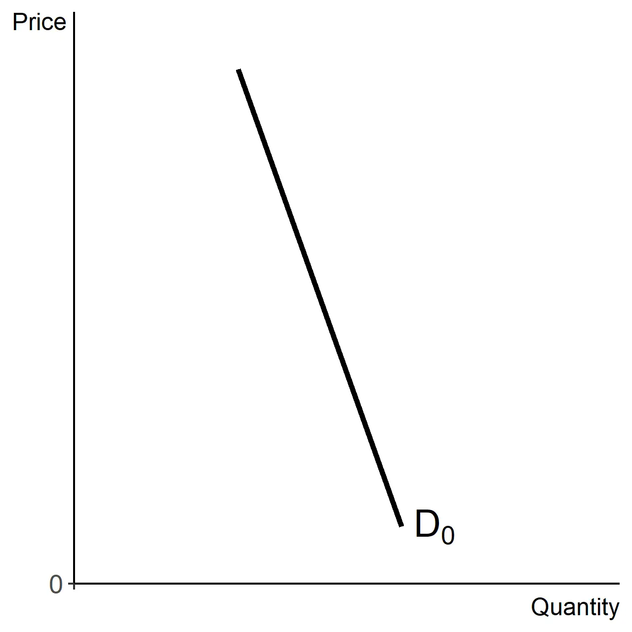
The law of demand ensures that demand curves slope downwards. If a price is lower, the quantity demanded should be higher, as long as nothing else changes. For AP Macroeconomics, it is enough to know that this comes from the good becoming relatively cheaper and a price decrease allowing consumers to afford to buy a larger amount of anything.

Any change in quantity demanded is a movement along a single demand curve.

Downward sloping demand curve, y-axis as price, x-axis as quantity.
Demand curve

If we change from a price decrease to a price increase, all of the explanations are simply reversed. Moving up the demand curve due to a price increase, leads to a lower quantity demanded.

In explanations and questions, there are two ways to discuss demand and they are both correct.

  • For each price, it tells us the quantity consumers wish to buy.
  • For each quantity, it tells us the highest amount that consumers would pay for that unit.

When demand is the focus, the second is usually more natural.

Supply

The other side of the market is the sellers. Their behavior is described by the supply curve.

Definitions
Supply curve / supply schedule
The relationship between price and quantity, holding all else equal (ceteris paribus). This will be either a graphed curve or a table of values.
Quantity supplied
A single point on a supply curve, representing the amount sellers are willing to sell at a specific price
Law of supply
If all else is held equal, as the price rises the quantity demanded rises…

As with demand, there is an important distinction between supply and the quantity supplied. Supply is shorthand for a single supply curve, giving a quantity supplied for different prices. The quantity supplied, is a single point on a single supply curve.

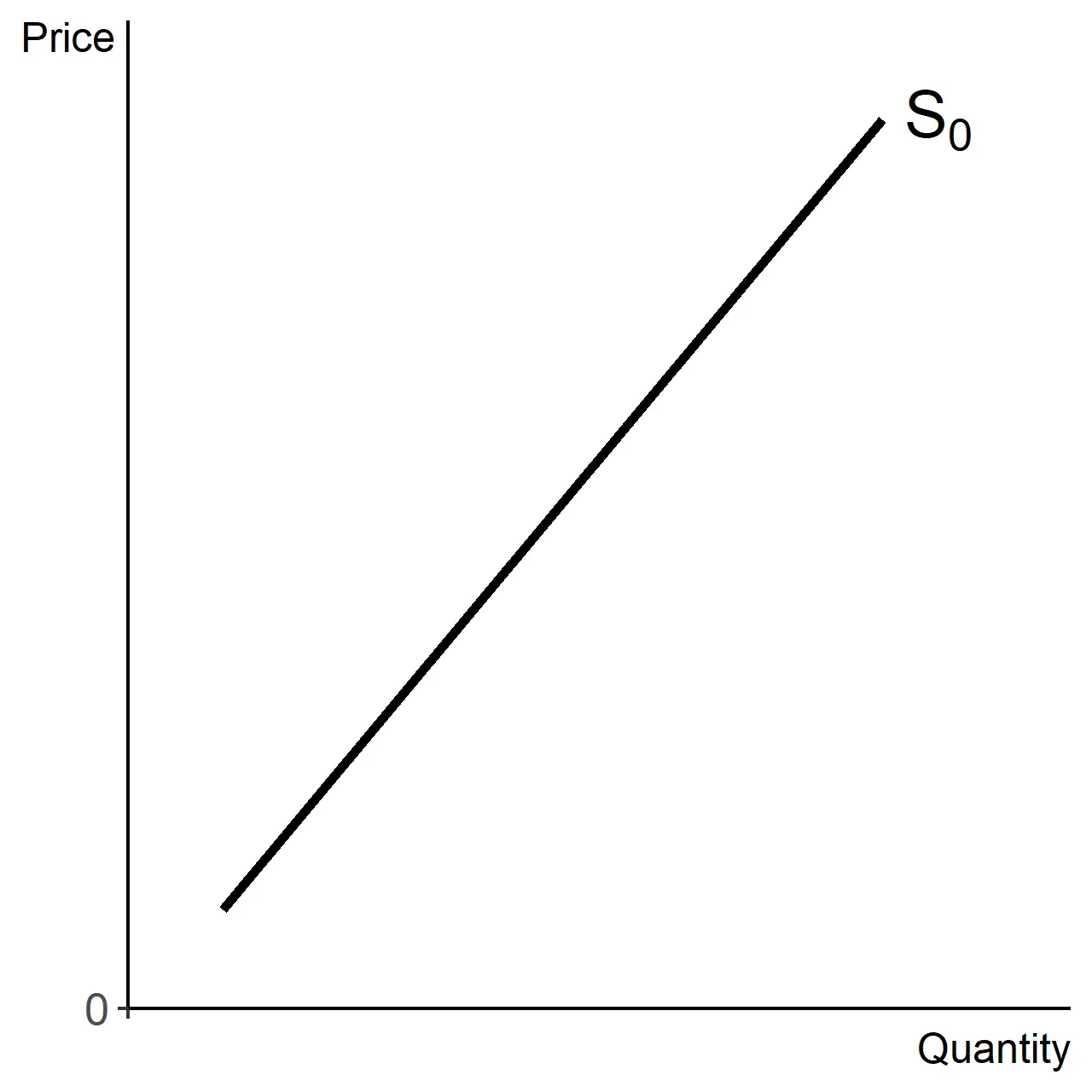
Just as the law of demand ensures that demand curves are downward sloping, the law of supply means that supply curves are upward sloping. Higher prices increase the quantity for sale and lower prices decrease the quantity for sale.

Upward sloping supply, y-axis as price, x-axis as quantity.
Supply curve

Supply also has two correct ways to describe it…

  • For each price, it tells us the quantity that will be put for sale
  • For each quantity, it tells us the lowest amount that a seller would accept for that specific unit.

When supply is the focus, the second is often more natural.

Our explanation of the law of supply is a lot simpler than the law of demand. As prices rise, resources have to be shifted to produce more of that good. This leads to the use of higher cost production options that were not worth pursuing at lower prices.

To return to our gas example, if there are enough customers, companies will add pumps to existing gas stations and for a large enough change more gas stations will be built. This explains why sometimes there are gas stations next to each other or even two stations from the same company on opposite sides of the same intersection. Prices must be high enough to support the cost of operating both stations.

That comment highlights an important idea, that supply curves are related to costs. In AP Microeconomics we go deeper into details about this, but for AP Macroeconomics that conceptual link is enough.

Market equilibrium

We can look at demand curves for individual consumers and we can add them up to get demand for any slice of consumers. For example people living in a specific state or country. We can also add demand for similar goods, say apples and bananas, to end up with demand for a broader definition of good, fruit.

The same holds for supply. We can look at supply curves for one factory, one firm, one location. We can look at supply for a single good and we can add together goods to end up with supply for a broader category.

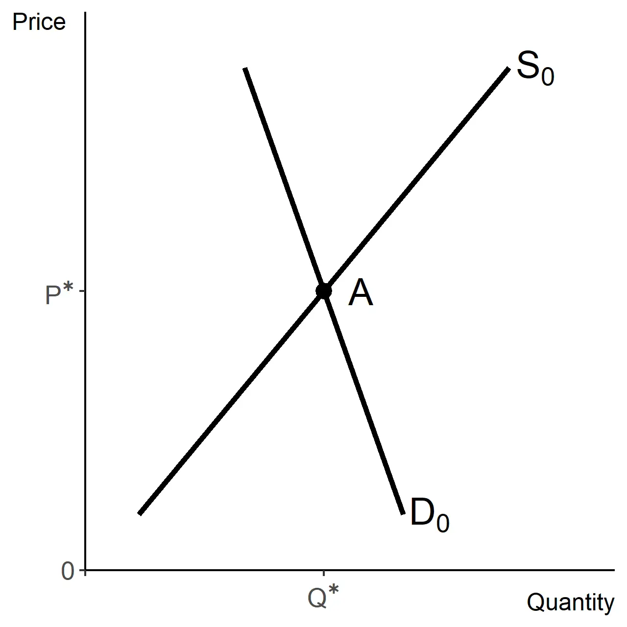
When we put supply and demand for one good together, we can find the equilibrium outcome. The market settles where the curves cross, point A. We will sometimes use P⋆ and Q⋆ to represent the equilibrium price and quantity, respectively.

Downward sloping demand, upward sloping supply. Equilibrium price and quantity where they cross.
Equilibrium

All buyers willing to pay P⋆ or more get to purchase the good or service. All sellers willing to sell for P⋆ or below, get to sell the good or service. This outcome is efficient in both senses, satisfying productive efficiency and allocative efficiency.

Prices are a reflection of incentives. For consumers, the incentives to purchase goods and gain benefits. For producers, the incentives to produce, adopt cost saving technologies and sell.

Thus in a competitive market, opportunity cost can always be viewed in terms of prices. That will not always be the most useful way to think of things, but it will always be a story we can tell.

Markets and Economic Systems

  • Market: system where buyers and sellers exchange goods/services
  • Competitive markets: many buyers/sellers, identical goods, no price control by individuals
  • Adam Smith’s “invisible hand”: self-interest leads to economic efficiency via price signals
  • Market failures: when markets don’t allocate efficiently (e.g., public goods, environmental protection)
  • Mixed economies: combine markets with government intervention due to market failures

Demand

  • Demand curve/schedule: relationship between price and quantity demanded, ceteris paribus
  • Quantity demanded: specific amount buyers will purchase at a given price (point on curve)
  • Law of demand: as price falls, quantity demanded rises (downward sloping curve)
  • Ceteris paribus: “all else equal”; isolates price-quantity relationship
  • Change in quantity demanded: movement along the demand curve

Supply

  • Supply curve/schedule: relationship between price and quantity supplied, ceteris paribus
  • Quantity supplied: specific amount sellers will offer at a given price (point on curve)
  • Law of supply: as price rises, quantity supplied rises (upward sloping curve)
  • Supply curves linked to production costs
  • Change in quantity supplied: movement along the supply curve

Market Equilibrium

  • Equilibrium: where supply and demand curves intersect
    • P⋆: equilibrium price
    • Q⋆: equilibrium quantity
  • At equilibrium: quantity supplied = quantity demanded
  • Market outcome is both productively and allocatively efficient
  • Prices reflect incentives and opportunity costs for buyers and sellers

Sign up for free to take 1 quiz question on this topic

Previous
Next  | 1.6 Demand and supply shifters
All rights reserved ©2016 - 2026 Achievable, Inc.

Markets

In our discussion of economic systems, the most commonly used word was market.

Besides being central to allocation in the real world, the concept is also listed by the College Board as one of the “Big Ideals” of AP Macroeconomics as a whole. A market can refer to a physical place where trade takes place or as a system where buyers and sellers exchange goods or services. When it is a system, we are looking to connect prices and quantities, which may be abbreviated by P and Q, respectively.

In macroeconomics we almost exclusively talk about competitive markets. These are markets where there are many buyers and sellers so no single participant controls the price and every unit of a good is identical. Demand represents buyers as a group and supply represents sellers as a group. Together they determine the equilibrium, or point where the price and quantity traded settles.

Adam Smith’s famous philosophy of the “invisible hand” says that many individuals pursuing their own self-interest pushes the economy towards economic efficiency. Prices give information to buyers and sellers, acting as signals that allow them to make the choices that are best for them and move resources to where they are most valued. Because of this, competitive markets naturally achieve allocative and productive efficiency.

The reason that mixed economies are so prevalent is market failures. A market failure refers to any case where the forces of supply and demand do not lead to an efficient allocation and government intervention is desirable. An easy example is environmental protection, benefits for which there are often no markets. Thus we treat the price as if it is zero and not enough is supplied. Another important example is a special kind of good called a public good, goods that may be used for free by many people at once. This includes things such as roads and national defense. Markets also fail to provide the socially optimal amount of these goods.

In AP Macroeconomics we will have cases later where a single actor, either the government or central bank, has a heavy influence on certain markets on their own. We can still consider these markets competitive, as long as the other side has many participants.

Regardless of categorization, we can use supply and demand analysis. We will just have to make some adjustments and be careful regarding our discussions.

Demand

Demand is the first piece of the market, the side of buyers. Our end goal is to be able to connect prices and quantities consumers are willing to buy. To get there we first must deal with the fact that there are factors other than price that impact how much consumers wish to buy.

To frame our concepts let us use the examples of a perfectly identical good: gasoline. For gas, we can imagine that we drive to work. For a large range of prices we will buy a fixed amount of gas for commuting. We also have necessary errands, such as buying groceries. As the price falls, we are more willing to drive for these other reasons. We may make smaller trips to the store rather than just one big trip on the weekends and start to add social trips, like driving to a friend’s house or going to a concert. For low enough prices, we start to consider road trips on weekends and vacations.

These non-price factors need not be the same for everyone and we will separate them more clearly and label them in the next subchapter. For now, we would like to set them aside.

In economics we accomplish this using the Latin phrase ceteris paribus. This can be translated as “all else equal,” “all else held constant,” or “other things unchanged.” All of these variations of describing the concept will be used frequently throughout the entire course. The point of focus for this market is the relationship between prices and quantities, so any other factor will be held constant.

This sets us up to describe the demand curve.

Definitions
Demand curve / demand schedule
The relationship between price and quantity, holding all else equal (ceteris paribus). This will be either a graphed curve or a table of values.
Quantity demanded
A single point on a demand curve, representing the amount buyers are willing to buy at a specific price.
The law of demand
If all else is held equal, as the price falls the quantity demanded rises. Similarly, as the price rises, the quantity demanded falls.

The distinction between the demand and the quantity demanded may seem trivial, but it is of critical importance. Demand refers to a single demand curve, which covers the entire set of desired choices by buyers. The quantity demanded is a single point on a demand curve.

The law of demand ensures that demand curves slope downwards. If a price is lower, the quantity demanded should be higher, as long as nothing else changes. For AP Macroeconomics, it is enough to know that this comes from the good becoming relatively cheaper and a price decrease allowing consumers to afford to buy a larger amount of anything.

Any change in quantity demanded is a movement along a single demand curve.

If we change from a price decrease to a price increase, all of the explanations are simply reversed. Moving up the demand curve due to a price increase, leads to a lower quantity demanded.

In explanations and questions, there are two ways to discuss demand and they are both correct.

  • For each price, it tells us the quantity consumers wish to buy.
  • For each quantity, it tells us the highest amount that consumers would pay for that unit.

When demand is the focus, the second is usually more natural.

Supply

The other side of the market is the sellers. Their behavior is described by the supply curve.

Definitions
Supply curve / supply schedule
The relationship between price and quantity, holding all else equal (ceteris paribus). This will be either a graphed curve or a table of values.
Quantity supplied
A single point on a supply curve, representing the amount sellers are willing to sell at a specific price
Law of supply
If all else is held equal, as the price rises the quantity demanded rises…

As with demand, there is an important distinction between supply and the quantity supplied. Supply is shorthand for a single supply curve, giving a quantity supplied for different prices. The quantity supplied, is a single point on a single supply curve.

Just as the law of demand ensures that demand curves are downward sloping, the law of supply means that supply curves are upward sloping. Higher prices increase the quantity for sale and lower prices decrease the quantity for sale.

Supply also has two correct ways to describe it…

  • For each price, it tells us the quantity that will be put for sale
  • For each quantity, it tells us the lowest amount that a seller would accept for that specific unit.

When supply is the focus, the second is often more natural.

Our explanation of the law of supply is a lot simpler than the law of demand. As prices rise, resources have to be shifted to produce more of that good. This leads to the use of higher cost production options that were not worth pursuing at lower prices.

To return to our gas example, if there are enough customers, companies will add pumps to existing gas stations and for a large enough change more gas stations will be built. This explains why sometimes there are gas stations next to each other or even two stations from the same company on opposite sides of the same intersection. Prices must be high enough to support the cost of operating both stations.

That comment highlights an important idea, that supply curves are related to costs. In AP Microeconomics we go deeper into details about this, but for AP Macroeconomics that conceptual link is enough.

Market equilibrium

We can look at demand curves for individual consumers and we can add them up to get demand for any slice of consumers. For example people living in a specific state or country. We can also add demand for similar goods, say apples and bananas, to end up with demand for a broader definition of good, fruit.

The same holds for supply. We can look at supply curves for one factory, one firm, one location. We can look at supply for a single good and we can add together goods to end up with supply for a broader category.

When we put supply and demand for one good together, we can find the equilibrium outcome. The market settles where the curves cross, point A. We will sometimes use P⋆ and Q⋆ to represent the equilibrium price and quantity, respectively.

All buyers willing to pay P⋆ or more get to purchase the good or service. All sellers willing to sell for P⋆ or below, get to sell the good or service. This outcome is efficient in both senses, satisfying productive efficiency and allocative efficiency.

Prices are a reflection of incentives. For consumers, the incentives to purchase goods and gain benefits. For producers, the incentives to produce, adopt cost saving technologies and sell.

Thus in a competitive market, opportunity cost can always be viewed in terms of prices. That will not always be the most useful way to think of things, but it will always be a story we can tell.

Key points

Markets and Economic Systems

  • Market: system where buyers and sellers exchange goods/services
  • Competitive markets: many buyers/sellers, identical goods, no price control by individuals
  • Adam Smith’s “invisible hand”: self-interest leads to economic efficiency via price signals
  • Market failures: when markets don’t allocate efficiently (e.g., public goods, environmental protection)
  • Mixed economies: combine markets with government intervention due to market failures

Demand

  • Demand curve/schedule: relationship between price and quantity demanded, ceteris paribus
  • Quantity demanded: specific amount buyers will purchase at a given price (point on curve)
  • Law of demand: as price falls, quantity demanded rises (downward sloping curve)
  • Ceteris paribus: “all else equal”; isolates price-quantity relationship
  • Change in quantity demanded: movement along the demand curve

Supply

  • Supply curve/schedule: relationship between price and quantity supplied, ceteris paribus
  • Quantity supplied: specific amount sellers will offer at a given price (point on curve)
  • Law of supply: as price rises, quantity supplied rises (upward sloping curve)
  • Supply curves linked to production costs
  • Change in quantity supplied: movement along the supply curve

Market Equilibrium

  • Equilibrium: where supply and demand curves intersect
    • P⋆: equilibrium price
    • Q⋆: equilibrium quantity
  • At equilibrium: quantity supplied = quantity demanded
  • Market outcome is both productively and allocatively efficient
  • Prices reflect incentives and opportunity costs for buyers and sellers

More from Core economic concepts

  • First principles
  • Opportunity cost examples
  • Ricardian trade
  • Macroeconomic choice
  • Demand and supply shifters