Linear approximations
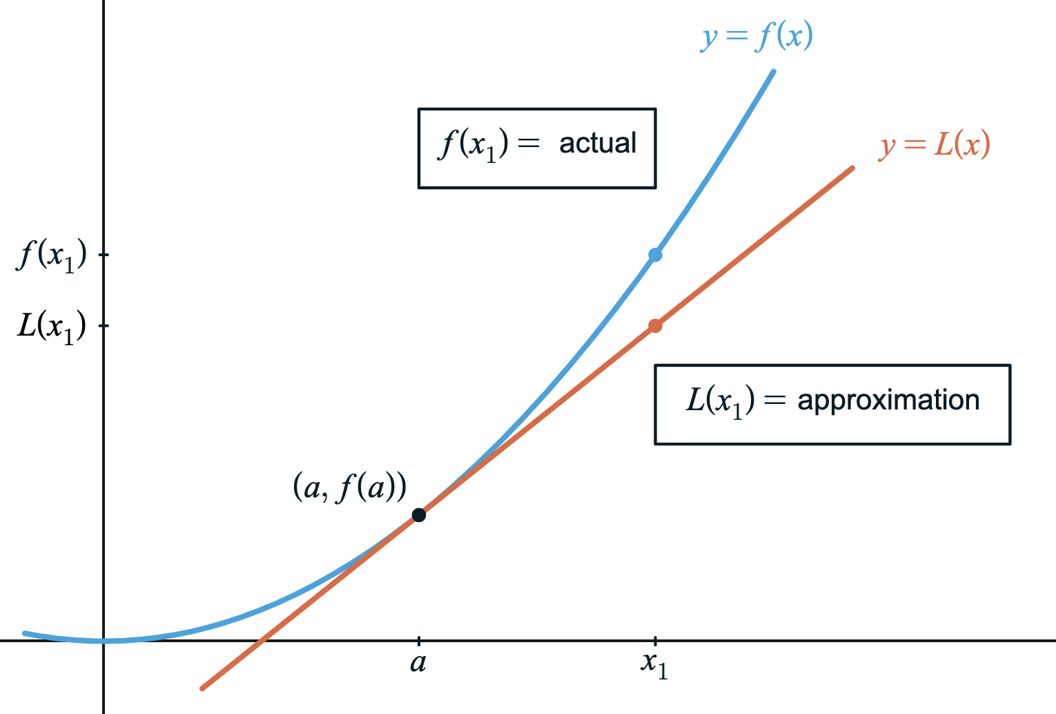
When a function is differentiable, its curve looks almost perfectly straight if you zoom in close enough to a single point. Because of this, the equation of a tangent line at a known point can be used approximate the values of the function for nearby inputs. This is called local linear approximation or tangent line approximation.
This formula is simply the equation of the tangent line to at . If an input is close to the center of approximation , then is a highly accurate estimate of the actual value .
Example
What is the approximate value of at using the tangent line to the graph at ?
- Bonus problem: Using the tangent line to the graph at instead, what is the approximate value of the same function at ?
Solution
This question essentially asks for the estimate of .
1. Find the point of tangency and the slope.
-
Point:
-
Slope:
2. Write the tangent line equation.
3. Compute the approximation .
Substitute :
In fact, the actual value is , so the linear estimate is very close.
Bonus problem solution
To write the tangent line equation to at instead, find the point and the slope:
-
Point:
-
Slope:
Then the equation of the tangent line is
The approximation for using this line instead is:
Notice how much further this is from the actual value of . Because the target value we chose to estimate () is further away from the anchor point where the tangent line was built (), the approximation is significantly less accurate.
Error analysis: Over vs. understimates
As demonstrated in the bonus problem, the accuracy of a linear approximation improves as the input gets closer to the anchor point .
Mathematically, error is defined as the difference between the actual value and the approximation:
By analyzing how is shaped near , we can determine whether the approximation is less than or greater than the actual value .
The 2nd derivative describes the concavity of a function - whether the graph bends upward or downward. More on concavity and its uses will come later. For now, keep these ideas in mind:
-
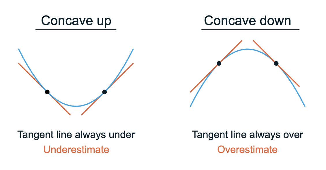
If , then is concave up (shaped “like a cup”).
- The tangent line lies below , so the linear approximation underestimates the actual value.
-
If , then is concave down (shaped “like a frown”).
- The tangent line lies above , so the linear approximation overestimates the actual value.
The image below shows this relationship between tangent lines and concavity.
Example
Let be the function defined by .
a) Use the line tangent to the graph of at to approximate .
b) Determine whether this approximation is an overestimate or an underestimate of the actual value of . Justify your answer.
Solutions
a) Use the line tangent to the graph of at to approximate .
1. Write the tangent line at .
-
Point:
-
Slope:
So the tangent line equation at is
2. Approximate .
Plug in :
b) Overestimate or underestimate?
To decide whether this is an overestimate or underestimate, find the 2nd derivative:
Since for all , is concave down for all in its domain. That means the tangent line lies above the curve, so the tangent line approximation overestimates the actual value.
A calculator confirms that , which is slightly less than the approximation of .
Challenge problem
Let be a twice-differentiable function. Selected values of and its derivative are given in the table below.
a) Must there be a value , for , such that ? Justify your answer.
b) Write an equation for the line tangent to the graph of at . Use this line to approximate the zero of .
Solutions
a) Must there be a value , for , such that ?
The wording of this problem suggests a textbook application of the Intermediate value theorem, where the target value . Your justification must state that the conditions are met:
-
Continuity:
- Since is twice-differentiable, and differentiability implies continuity, is guaranteed to be continuous on .
-
is between and :
- From the table, and
- Since , this condition has been met.
Therefore, the Intermediate value theorem guarantees a in the open interval such that .
b) Write an equation for the line tangent to the graph of at . Use this line to approximate the zero of .
The tangent line equation at is
A zero, or root, of is where the function crosses the -axis, meaning . While a tangent line is usually used to approximate a -value, here we work “backwards” to find the value of for which :
Therefore, the tangent line approximates the zero of to be at . Notice how this approximation falls perfectly within the open interval guaranteed by the IVT in part (a).