Important theorems
In addition to the Intermediate value theorem (from section 1.6 on Continuity), there are two other main existence theorems in calculus: the Mean value theorem (with Rolle’s theorem as a special case) and the Extreme value theorem.
Mean value theorem
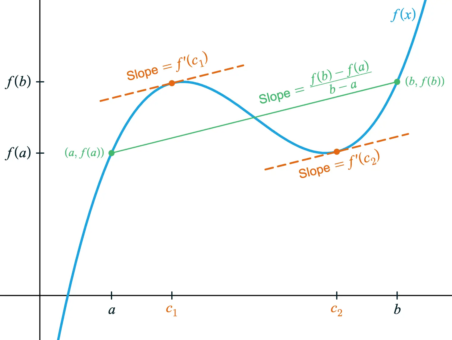
As shown in the figure below, function satisfies the Mean value theorem at two values, and .
At these points, the slopes of the tangent lines, and , are equal to the slope of the secant line passing through the endpoints of the interval and .
Examples
- Determine if the Mean value theorem can be applied to on the interval given and if so, find the values of that satisfy the theorem.
a) on
b) on
c) on
Solutions
a) on
is a polynomial, which is continuous and differentiable for all , so the MVT applies.
Find the average rate of change of over :
Differentiate :
Set the derivative equal to the average rate of change:
So is the point where the instantaneous rate of change equals the average rate of change.
b) on
is a polynomial, so the MVT applies.
Find the average rate of change over :
Differentiate :
Set the derivative equal to the average rate of change:
Because must be in the open interval , we eliminate . So is the only value that satisfies the MVT.
c) on
is the upper half of a circle of radius .
1. Continuity
Although the semicircle is not defined past the left endpoint for , continuity on a closed interval only requires:
- Continuity from the right at the left endpoint:
- Continuity from the left at the right endpoint:
So the 1st condition of the MVT is satisfied.
2. Differentiability
Even though does not exist, the MVT only requires differentiability on the open interval . Since is differentiable on the entire interval , the 2nd condition is also satisfied.
Find the average rate of change over :
Differentiate :
Set the derivative equal to the average rate of change:
is the only solution that satisfies the MVT because it lies within the open interval .
Rolle’s theorem
Rolle’s theorem is a special case of the Mean value theorem where the function starts and ends at the same value, meaning . In that situation, Rolle’s theorem guarantees at least one point in the interval where the tangent line is horizontal (a derivative of ).
Examples
Determine if Rolle’s theorem can be applied to on the closed interval given and if so, find the values of that satisfy the theorem.
a) on
b) on
c) on
Solutions
a) on
is a polynomial so the first two conditions of Rolle’s theorem are met.
For the 3rd condition, check:
Since , Rolle’s theorem applies.
Next, differentiate :
Set :
This matches the graph of , which has a horizontal tangent line at .
b) on
is a rational function and is discontinuous at , which lies in the interval . Since the continuity condition fails, Rolle’s theorem cannot be applied. A horizontal tangent might still exist in the interval, but the theorem does not guarantee one.
c) on
is continuous on , but it is not differentiable at , which is inside the interval. Since differentiability on fails, Rolle’s theorem does not apply. In fact, there is no point on this graph where the tangent line is horizontal.
Extreme value theorem
The extreme value theorem guarantees that a continuous function has both a highest value and a lowest value on a closed interval. These absolute extrema can occur at interior points or at the endpoints.
The Candidates Test is the practical application of the EVT, used to find the absolute maximum and minimum on an interval:
-
Verify continuity on the interval: If there are any breaks, jumps, or asymptotes, the EVT is not applicable.
-
Find critical points: Solve or determine where it is undefined within .
-
Evaluate function values of the candidates: Compute at the critical points and at the endpoints - and .
-
Compare function values: The largest function value is the absolute maximum and the smallest is the absolute minimum on that interval.
Examples
- Find the absolute extrema of on .
1. Verify continuity
is a polynomial, so it’s continuous.
2. Find critical points
Solve :
3. Evaluate function values
At the critical point ,
At the endpoints,
4. Compare function values
The absolute maximum is , which occurs at .
The absolute minimum is , which occurs at .
- Find the absolute extrema of
on .
Solution
1. Verify continuity
This rational function has a vertical asymptote at , but is not in . So is continuous on the given interval.
2. Find critical points
Since for all in , there are no critical points in the interval.
3. Evaluate function values
With no critical points, evaluate only the endpoints:
4. Compare function values
The absolute minimum is at .
The absolute maximum is at .