


Achievable logoAchievable logo
FE Civil
Sign in
Sign up
Purchase
Textbook
Practice exams
Support
How it works
Exam catalog
Mountain with a flag at the peak
Textbook
Introduction
1. Mathematics
2. Combinatorics, probability and statistics
3. Engineering economics
4. Statics
5. Materials
6. Dynamics
7. Mechanics of materials
8. Fluid mechanics
9. Soil mechanics
10. Structural engineering
11. Concrete structure design
12. Water resources engineering
13. Environmental engineering
14. Transportation engineering
15. Surveying, construction, ethics and professional practice
16. Wrapping up
(change me)
Achievable logoAchievable logo
3. Engineering economics
Achievable FE Civil
Our FE Civil course is currently in development and is a work-in-progress.

Engineering economics

10 min read
Font
Discuss
Share
Feedback

This chapter covers the following topics:

  • Types of cash flow
  • The year-end accounting convention
  • Nonannual compounding
  • Present worth
  • Principal in a sinking fund
  • Capitalized cost
  • Equivalent uniform annual cost
  • Depreciation
  • Sum of years digits method
  • Units of production method
  • Modified accelerated cost recovery system
  • Tax issues
  • Bonds
  • Break-even analysis
  • Benefit-cost analysis

The primary objective of engineering economic analysis is to compare economic alternatives based on cost.

Types of cash flow

Definitions

Cash flow refers to the movement of money into or out of a project or investment.

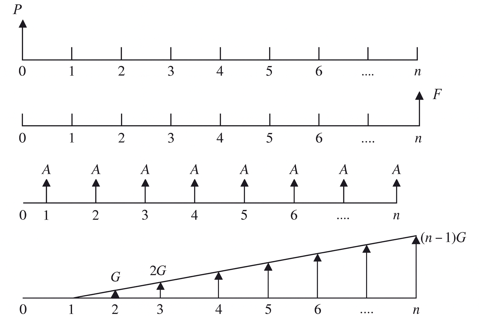
In engineering economics, we often model real cash flows using a few idealized patterns. The four types discussed in this chapter are:

Types:

  • Present value (P): a one-time cash flow that occurs now (i.e., at t=0).
  • Future value (F): a one-time cash flow that occurs after a finite duration (t=n).
  • Annuity (A): a constant cash flow that starts at t=1 and repeats for n time periods.
  • Gradient series (G): a uniformly increasing (arithmetic) finite cash flow series that has value zero at t=1, value G at t=2, 2G at t=3, and so on, ending at a value (n−1)G at t=n.
A schematic showing different types of cash-flow distributions along a time axis, including single lump sums, uniform series, and a linearly increasing (arithmetic gradient) series.
Types of cash flows

Example:

A machine costs $10,000, generates $3,000/year for 5 years, and has a salvage value of $1,000.

Year-end accounting convention

Definitions

All cash flows occur at the end of each year for simplicity.

To keep calculations consistent, we assume cash flows occur at the end of each year. This is the year-end accounting convention.

The equations in this section rely on the time value of money: money today can grow over time if it earns interest. That growth occurs through compounding at a rate of return.

In engineering economic analysis, the rate of return is often the MARR (Minimum Attractive Rate of Return). In the formulas, MARR is represented by i. MARR is the lowest rate of return an investor is willing to accept, given the investment’s risk and the opportunity to earn returns elsewhere.

Two compounding models are used:

  1. Discrete compounding: interest is added at regular time intervals.
  2. Continuous compounding: the limit as the number of compounding periods becomes infinitely large (n→∞).

Note: For continuous compounding, gradient series formulas are not included because they are not meaningful in that case.

The equations below convert money values across time using these variables:

  • P - present worth (single lump sum).
  • A - an annuity (constant installment at the end of every period).
  • F - future worth (single lump sum).
  • G - gradient series starting at zero for the first period and increasing by constant increment G every period.
  • i - nominal interest rate per period (MARR). This is often stated as a percentage, but you must use a decimal value in the equations.
  • n - the number of compounding intervals.

Single payment compound - converts to F, given P

Symbol: F=P(F/P,i,n)

  • Discrete compounding:

    F=P(1+i)n

  • Continuous compounding:

    F=Pein

Single payment present worth - converts to P, given F

Symbol: P=F(P/F,i,n)

  • Discrete compounding:

    P=(1+i)nF​

  • Continuous compounding:

    P=Fe−in

Uniform series sinking fund - converts to A, given F

Symbol: A=F(A/F,i,n)

  • Discrete compounding:

    A=F⋅(1+i)n−1i​

  • Continuous compounding:

    A=F⋅ein−1iein​

Capital recovery - converts to A, given P

Symbol: A=P(A/P,i,n)

  • Discrete compounding:

    A=P⋅(1+i)n−1i(1+i)n​

  • Continuous compounding:

    A=P⋅ein−1iein​

Uniform series compound - converts to F, given A

Symbol: F=A(F/A,i,n)

  • Discrete compounding:

    F=A⋅i(1+i)n−1​

  • Continuous compounding:

    F=A⋅iein−1​

Uniform series present worth - converts to P, given A

Symbol: P=A(P/A,i,n)

  • Discrete compounding:

    P=A⋅i(1+i)n(1+i)n−1​

  • Continuous compounding:

    P=A⋅ieinein−1​

Uniform gradient present worth - converts to P, given G

Symbol: P=G(P/G,i,n)

  • Discrete compounding:

    P=G⋅(i(1+i)n(1+i)n−1​−(1+i)nn​)

  • Continuous compounding:

    Undefined

Uniform gradient future worth - converts to F, given G

Symbol: F=G(F/G,i,n)

  • Discrete compounding:

    F=G⋅(i(1+i)n−1​−n)

  • Continuous compounding:

    Undefined

Uniform gradient uniform series - converts to A, given G

Symbol: A=G(A/G,i,n)

  • Discrete compounding:

    A=G⋅(i1​−(1+i)n−1n​)

  • Continuous compounding:

    Undefined

Interest rate tables are based on these relationships. For detailed tables, refer to the FE Handbook.

Nonannual compounding

Definitions

Interest can be compounded more frequently than annually.

Interest can be compounded more frequently than once per year (for example, monthly or quarterly). The interest rate tables are built around a specific time period, so you need the interest rate per period to use them correctly.

For example, if the time period is 3 years and the effective annual interest rate is 6%, then the table gives (P/F, i=6%, n=3) = 0.8396.

However, if time is measured in months (for example, 36 months) while the interest rate is still given as an effective annual rate of 6%, you can’t use the annual tables directly. The compounding period has changed.

In that case, convert the annual effective rate to an equivalent monthly interest rate, iM​, meaning the monthly rate that compounds to 6% over 12 months:

(1+iM​)12=1.06⇒iM​=0.00487(0.487%)

Since tables typically won’t include i=0.00487, you use the formula to compute the (P/F, i=0.00487, n=36) factor. That factor equals 0.8396, matching the 3-year calculation because 6% was given as an effective annual rate.

If the 6% were instead a nominal annual rate, the monthly rate would be 6%÷12=0.5% or 0.005. Then the (P/F, i=0.005, n=36) factor would be different (specifically, 0.8356).

Formula:

F=P(1+mi​)n⋅m

Where:

  • F = Future value
  • P = Present value
  • i = Annual interest rate
  • m = Compounding periods per year
  • n = Number of years

Example:

Invest $1,000 at 8% compounded quarterly for 3 years:

F=1000(1+40.08​)3⋅4=1000(1.02)12=1268.24

Present worth (P)

Definitions

Current value of future cash flows.

Present worth converts future cash flows into an equivalent value at time t=0 using an interest rate i.

Formula:

P=∑(1+i)tCFt​​

Where:

  • CFt​ = Cash flow at year t
  • i = Interest rate
  • t = Time period

Example:

Receive $500 annually for 3 years at 10%:

P=1.1500​+1.12500​+1.13500​=500(2.4869)=1243.45

Principal in a sinking fund

Used to accumulate a future sum through periodic payments.

Formula:

A=(1+i)n−1F⋅i​

Where:

  • A = Annual deposit
  • F = Future value
  • i = Interest rate
  • n = Number of periods

Example:

Save $10,000 in 5 years at 6% interest:

A=(1.06)5−110000⋅0.06​=0.3382600​=1773.96

Capitalized cost

Definitions

Used for projects with infinite lives.

Capitalized cost is used when a project is assumed to continue indefinitely (an infinite life). It expresses the project’s cost as a single present-worth amount.

Formula:

CC=P+iA​

Where:

  • P = Initial cost
  • A = Annual cost
  • i = Interest rate

Example:

A project costs $50,000 initially and $2,000/year to maintain at 5%:

CC=50000+0.052000​=50000+40000=90000

Equivalent uniform annual cost (EUAC)

Converts all costs into an equivalent annual amount.

Formula:

EUAC=P(A/P,i,n)+A

Where:

  • A = Annual cost
  • P(A/P,i,n) = Capital recovery factor

Depreciation

Definitions

Reduction in value of an asset over time.

Depreciation models how an asset’s value is allocated (or reduced) over its useful life.

General formula (straight-line):

D=nP−S​

Where:

  • D = Annual depreciation
  • P = Initial cost
  • S = Salvage value
  • n = Useful life

Sum-of-years-digits (SYD) method

Definitions

Accelerated depreciation method.

The SYD method accelerates depreciation by assigning larger depreciation amounts in earlier years.

Formula:

Dt​=2n(n+1)​(n−t+1)​(P−S)

Where:

  • t = Year
  • n = Useful life

Units of production method

Depreciation based on usage rather than time.

Formula:

D=Total units(P−S)​×Units used in year

Modified accelerated cost recovery system (MACRS)

Used in U.S. tax code for accelerated depreciation.

  • Based on IRS tables.
  • Assumes half-year convention.

Example: 5-year property with 20% depreciation in Year 1.

Tax issues

Key concepts:

  • Depreciation is tax-deductible.

  • Taxable Income:

    TI=Revenue−Expenses−Depreciation

  • Taxes:

    Tax=TI×Tax Rate

Bonds

Definitions

Debt instruments used to raise capital.

A bond’s value today is the present worth of its coupon payments plus the present worth of its face value paid at maturity.

Bond Valuation:

P=∑(1+i)tC​+(1+i)nF​

Where:

  • P = Bond price
  • C = Coupon payment
  • F = Face value
  • i = Market interest rate
  • n = Maturity

Break-even analysis

Definitions

Finds point where revenue equals costs.

Break-even analysis finds the output level where total revenue equals total cost.

Formula:

Q=P−VF​

Where:

  • Q = Break-even quantity
  • F = Fixed cost
  • P = Price per unit
  • V = Variable cost per unit

Benefit-Cost (B/C) analysis

Definitions

Used in public project evaluation.

Benefit-cost analysis compares the present worth of benefits to the present worth of costs.

Formula:

B/C=Present worth of costsPresent worth of benefits​

  • If B/C>1, project is acceptable.

Types of cash flow

  • Four types: Present value (P), Future value (F), Annuity (A), Gradient series (G)
  • Each type models a different cash flow pattern over time
  • Example: machine purchase with annual returns and salvage value

Year-end accounting convention

  • Assume all cash flows occur at year-end
  • Time value of money: money grows via compounding at rate i (often MARR)
  • Two compounding models: discrete and continuous

Time value of money formulas

  • Single payment compound: F=P(1+i)n (discrete), F=Pein (continuous)
  • Present worth: P=F/(1+i)n (discrete), P=Fe−in (continuous)
  • Uniform series and gradient series formulas for converting between P, A, F, G
  • Interest rate tables based on these relationships

Nonannual compounding

  • Interest can be compounded more than once per year (e.g., monthly)
  • Convert annual rate to per-period rate for correct calculations
  • Formula: F=P(1+mi​)n⋅m

Present worth (P)

  • Present value of future cash flows discounted at rate i
  • Formula: P=∑(1+i)tCFt​​

Principal in a sinking fund

  • Accumulate a future sum via periodic payments
  • Formula: A=(1+i)n−1F⋅i​

Capitalized cost

  • Used for projects with infinite lives
  • Formula: CC=P+iA​

Equivalent uniform annual cost (EUAC)

  • Converts all costs to an equivalent annual amount
  • Formula: EUAC=P(A/P,i,n)+A

Depreciation

  • Models reduction in asset value over time
  • Straight-line formula: D=nP−S​

Sum-of-years-digits (SYD) method

  • Accelerated depreciation: higher in early years
  • Formula: Dt​=2n(n+1)​(n−t+1)​(P−S)

Units of production method

  • Depreciation based on usage, not time
  • Formula: D=Total units(P−S)​×Units used in year

Modified accelerated cost recovery system (MACRS)

  • U.S. tax code accelerated depreciation method
  • Uses IRS tables and half-year convention

Tax issues

  • Depreciation is tax-deductible
  • Taxable income: TI=Revenue−Expenses−Depreciation
  • Taxes owed: Tax=TI×Tax Rate

Bonds

  • Bonds are debt instruments; value is present worth of coupons plus face value
  • Formula: P=∑(1+i)tC​+(1+i)nF​

Break-even analysis

  • Finds output level where revenue equals costs
  • Formula: Q=P−VF​

Benefit-Cost (B/C) analysis

  • Compares present worth of benefits to costs
  • Accept project if B/C>1

Sign up for free to take 5 quiz questions on this topic

Previous
Next  | 4. Statics
All rights reserved ©2016 - 2026 Achievable, Inc.

Engineering economics

This chapter covers the following topics:

  • Types of cash flow
  • The year-end accounting convention
  • Nonannual compounding
  • Present worth
  • Principal in a sinking fund
  • Capitalized cost
  • Equivalent uniform annual cost
  • Depreciation
  • Sum of years digits method
  • Units of production method
  • Modified accelerated cost recovery system
  • Tax issues
  • Bonds
  • Break-even analysis
  • Benefit-cost analysis

The primary objective of engineering economic analysis is to compare economic alternatives based on cost.

Types of cash flow

Definitions

Cash flow refers to the movement of money into or out of a project or investment.

In engineering economics, we often model real cash flows using a few idealized patterns. The four types discussed in this chapter are:

Types:

  • Present value (P): a one-time cash flow that occurs now (i.e., at t=0).
  • Future value (F): a one-time cash flow that occurs after a finite duration (t=n).
  • Annuity (A): a constant cash flow that starts at t=1 and repeats for n time periods.
  • Gradient series (G): a uniformly increasing (arithmetic) finite cash flow series that has value zero at t=1, value G at t=2, 2G at t=3, and so on, ending at a value (n−1)G at t=n.

Example:

A machine costs $10,000, generates $3,000/year for 5 years, and has a salvage value of $1,000.

Year-end accounting convention

Definitions

All cash flows occur at the end of each year for simplicity.

To keep calculations consistent, we assume cash flows occur at the end of each year. This is the year-end accounting convention.

The equations in this section rely on the time value of money: money today can grow over time if it earns interest. That growth occurs through compounding at a rate of return.

In engineering economic analysis, the rate of return is often the MARR (Minimum Attractive Rate of Return). In the formulas, MARR is represented by i. MARR is the lowest rate of return an investor is willing to accept, given the investment’s risk and the opportunity to earn returns elsewhere.

Two compounding models are used:

  1. Discrete compounding: interest is added at regular time intervals.
  2. Continuous compounding: the limit as the number of compounding periods becomes infinitely large (n→∞).

Note: For continuous compounding, gradient series formulas are not included because they are not meaningful in that case.

The equations below convert money values across time using these variables:

  • P - present worth (single lump sum).
  • A - an annuity (constant installment at the end of every period).
  • F - future worth (single lump sum).
  • G - gradient series starting at zero for the first period and increasing by constant increment G every period.
  • i - nominal interest rate per period (MARR). This is often stated as a percentage, but you must use a decimal value in the equations.
  • n - the number of compounding intervals.

Single payment compound - converts to F, given P

Symbol: F=P(F/P,i,n)

  • Discrete compounding:

    F=P(1+i)n

  • Continuous compounding:

    F=Pein

Single payment present worth - converts to P, given F

Symbol: P=F(P/F,i,n)

  • Discrete compounding:

    P=(1+i)nF​

  • Continuous compounding:

    P=Fe−in

Uniform series sinking fund - converts to A, given F

Symbol: A=F(A/F,i,n)

  • Discrete compounding:

    A=F⋅(1+i)n−1i​

  • Continuous compounding:

    A=F⋅ein−1iein​

Capital recovery - converts to A, given P

Symbol: A=P(A/P,i,n)

  • Discrete compounding:

    A=P⋅(1+i)n−1i(1+i)n​

  • Continuous compounding:

    A=P⋅ein−1iein​

Uniform series compound - converts to F, given A

Symbol: F=A(F/A,i,n)

  • Discrete compounding:

    F=A⋅i(1+i)n−1​

  • Continuous compounding:

    F=A⋅iein−1​

Uniform series present worth - converts to P, given A

Symbol: P=A(P/A,i,n)

  • Discrete compounding:

    P=A⋅i(1+i)n(1+i)n−1​

  • Continuous compounding:

    P=A⋅ieinein−1​

Uniform gradient present worth - converts to P, given G

Symbol: P=G(P/G,i,n)

  • Discrete compounding:

    P=G⋅(i(1+i)n(1+i)n−1​−(1+i)nn​)

  • Continuous compounding:

    Undefined

Uniform gradient future worth - converts to F, given G

Symbol: F=G(F/G,i,n)

  • Discrete compounding:

    F=G⋅(i(1+i)n−1​−n)

  • Continuous compounding:

    Undefined

Uniform gradient uniform series - converts to A, given G

Symbol: A=G(A/G,i,n)

  • Discrete compounding:

    A=G⋅(i1​−(1+i)n−1n​)

  • Continuous compounding:

    Undefined

Interest rate tables are based on these relationships. For detailed tables, refer to the FE Handbook.

Nonannual compounding

Definitions

Interest can be compounded more frequently than annually.

Interest can be compounded more frequently than once per year (for example, monthly or quarterly). The interest rate tables are built around a specific time period, so you need the interest rate per period to use them correctly.

For example, if the time period is 3 years and the effective annual interest rate is 6%, then the table gives (P/F, i=6%, n=3) = 0.8396.

However, if time is measured in months (for example, 36 months) while the interest rate is still given as an effective annual rate of 6%, you can’t use the annual tables directly. The compounding period has changed.

In that case, convert the annual effective rate to an equivalent monthly interest rate, iM​, meaning the monthly rate that compounds to 6% over 12 months:

(1+iM​)12=1.06⇒iM​=0.00487(0.487%)

Since tables typically won’t include i=0.00487, you use the formula to compute the (P/F, i=0.00487, n=36) factor. That factor equals 0.8396, matching the 3-year calculation because 6% was given as an effective annual rate.

If the 6% were instead a nominal annual rate, the monthly rate would be 6%÷12=0.5% or 0.005. Then the (P/F, i=0.005, n=36) factor would be different (specifically, 0.8356).

Formula:

F=P(1+mi​)n⋅m

Where:

  • F = Future value
  • P = Present value
  • i = Annual interest rate
  • m = Compounding periods per year
  • n = Number of years

Example:

Invest $1,000 at 8% compounded quarterly for 3 years:

F=1000(1+40.08​)3⋅4=1000(1.02)12=1268.24

Present worth (P)

Definitions

Current value of future cash flows.

Present worth converts future cash flows into an equivalent value at time t=0 using an interest rate i.

Formula:

P=∑(1+i)tCFt​​

Where:

  • CFt​ = Cash flow at year t
  • i = Interest rate
  • t = Time period

Example:

Receive $500 annually for 3 years at 10%:

P=1.1500​+1.12500​+1.13500​=500(2.4869)=1243.45

Principal in a sinking fund

Used to accumulate a future sum through periodic payments.

Formula:

A=(1+i)n−1F⋅i​

Where:

  • A = Annual deposit
  • F = Future value
  • i = Interest rate
  • n = Number of periods

Example:

Save $10,000 in 5 years at 6% interest:

A=(1.06)5−110000⋅0.06​=0.3382600​=1773.96

Capitalized cost

Definitions

Used for projects with infinite lives.

Capitalized cost is used when a project is assumed to continue indefinitely (an infinite life). It expresses the project’s cost as a single present-worth amount.

Formula:

CC=P+iA​

Where:

  • P = Initial cost
  • A = Annual cost
  • i = Interest rate

Example:

A project costs $50,000 initially and $2,000/year to maintain at 5%:

CC=50000+0.052000​=50000+40000=90000

Equivalent uniform annual cost (EUAC)

Converts all costs into an equivalent annual amount.

Formula:

EUAC=P(A/P,i,n)+A

Where:

  • A = Annual cost
  • P(A/P,i,n) = Capital recovery factor

Depreciation

Definitions

Reduction in value of an asset over time.

Depreciation models how an asset’s value is allocated (or reduced) over its useful life.

General formula (straight-line):

D=nP−S​

Where:

  • D = Annual depreciation
  • P = Initial cost
  • S = Salvage value
  • n = Useful life

Sum-of-years-digits (SYD) method

Definitions

Accelerated depreciation method.

The SYD method accelerates depreciation by assigning larger depreciation amounts in earlier years.

Formula:

Dt​=2n(n+1)​(n−t+1)​(P−S)

Where:

  • t = Year
  • n = Useful life

Units of production method

Depreciation based on usage rather than time.

Formula:

D=Total units(P−S)​×Units used in year

Modified accelerated cost recovery system (MACRS)

Used in U.S. tax code for accelerated depreciation.

  • Based on IRS tables.
  • Assumes half-year convention.

Example: 5-year property with 20% depreciation in Year 1.

Tax issues

Key concepts:

  • Depreciation is tax-deductible.

  • Taxable Income:

    TI=Revenue−Expenses−Depreciation

  • Taxes:

    Tax=TI×Tax Rate

Bonds

Definitions

Debt instruments used to raise capital.

A bond’s value today is the present worth of its coupon payments plus the present worth of its face value paid at maturity.

Bond Valuation:

P=∑(1+i)tC​+(1+i)nF​

Where:

  • P = Bond price
  • C = Coupon payment
  • F = Face value
  • i = Market interest rate
  • n = Maturity

Break-even analysis

Definitions

Finds point where revenue equals costs.

Break-even analysis finds the output level where total revenue equals total cost.

Formula:

Q=P−VF​

Where:

  • Q = Break-even quantity
  • F = Fixed cost
  • P = Price per unit
  • V = Variable cost per unit

Benefit-Cost (B/C) analysis

Definitions

Used in public project evaluation.

Benefit-cost analysis compares the present worth of benefits to the present worth of costs.

Formula:

B/C=Present worth of costsPresent worth of benefits​

  • If B/C>1, project is acceptable.
Key points

Types of cash flow

  • Four types: Present value (P), Future value (F), Annuity (A), Gradient series (G)
  • Each type models a different cash flow pattern over time
  • Example: machine purchase with annual returns and salvage value

Year-end accounting convention

  • Assume all cash flows occur at year-end
  • Time value of money: money grows via compounding at rate i (often MARR)
  • Two compounding models: discrete and continuous

Time value of money formulas

  • Single payment compound: F=P(1+i)n (discrete), F=Pein (continuous)
  • Present worth: P=F/(1+i)n (discrete), P=Fe−in (continuous)
  • Uniform series and gradient series formulas for converting between P, A, F, G
  • Interest rate tables based on these relationships

Nonannual compounding

  • Interest can be compounded more than once per year (e.g., monthly)
  • Convert annual rate to per-period rate for correct calculations
  • Formula: F=P(1+mi​)n⋅m

Present worth (P)

  • Present value of future cash flows discounted at rate i
  • Formula: P=∑(1+i)tCFt​​

Principal in a sinking fund

  • Accumulate a future sum via periodic payments
  • Formula: A=(1+i)n−1F⋅i​

Capitalized cost

  • Used for projects with infinite lives
  • Formula: CC=P+iA​

Equivalent uniform annual cost (EUAC)

  • Converts all costs to an equivalent annual amount
  • Formula: EUAC=P(A/P,i,n)+A

Depreciation

  • Models reduction in asset value over time
  • Straight-line formula: D=nP−S​

Sum-of-years-digits (SYD) method

  • Accelerated depreciation: higher in early years
  • Formula: Dt​=2n(n+1)​(n−t+1)​(P−S)

Units of production method

  • Depreciation based on usage, not time
  • Formula: D=Total units(P−S)​×Units used in year

Modified accelerated cost recovery system (MACRS)

  • U.S. tax code accelerated depreciation method
  • Uses IRS tables and half-year convention

Tax issues

  • Depreciation is tax-deductible
  • Taxable income: TI=Revenue−Expenses−Depreciation
  • Taxes owed: Tax=TI×Tax Rate

Bonds

  • Bonds are debt instruments; value is present worth of coupons plus face value
  • Formula: P=∑(1+i)tC​+(1+i)nF​

Break-even analysis

  • Finds output level where revenue equals costs
  • Formula: Q=P−VF​

Benefit-Cost (B/C) analysis

  • Compares present worth of benefits to costs
  • Accept project if B/C>1

Related readings

  • Introduction
  • Statics
  • Dynamics
  • Mechanics of materials
  • Structural engineering