




This browser is too old to run Achievable.

Update it, or open this page in a current version of Chrome, Safari, Firefox or Edge. On an iPhone or iPad, update iOS: every browser there runs on the version of Safari that comes with it.

Achievable logoAchievable logo
CMA Part 1
Sign in
Sign up
Purchase
Textbook
Practice exams
Support
How it works
Resources
Exam catalog
Mountain with a flag at the peak
Textbook
Introduction
1. External financial reporting decisions
2. Planning, budgeting, and forecasting
3. Performance management
4. Cost management
5. Internal control
6. Technology and analytics
Wrapping up
Achievable logoAchievable logo
3.1.4.6.3 Production volume variance
Achievable CMA Part 1
3. Cost and variance measures
3.1. Management by exception and standard cost systems
3.1.4. Fixed overhead (FOH) cost variance
Our CMA Part 1 course is currently in development and is a work-in-progress.

Production volume variance

6 min read
Font
Discuss
Share
Feedback
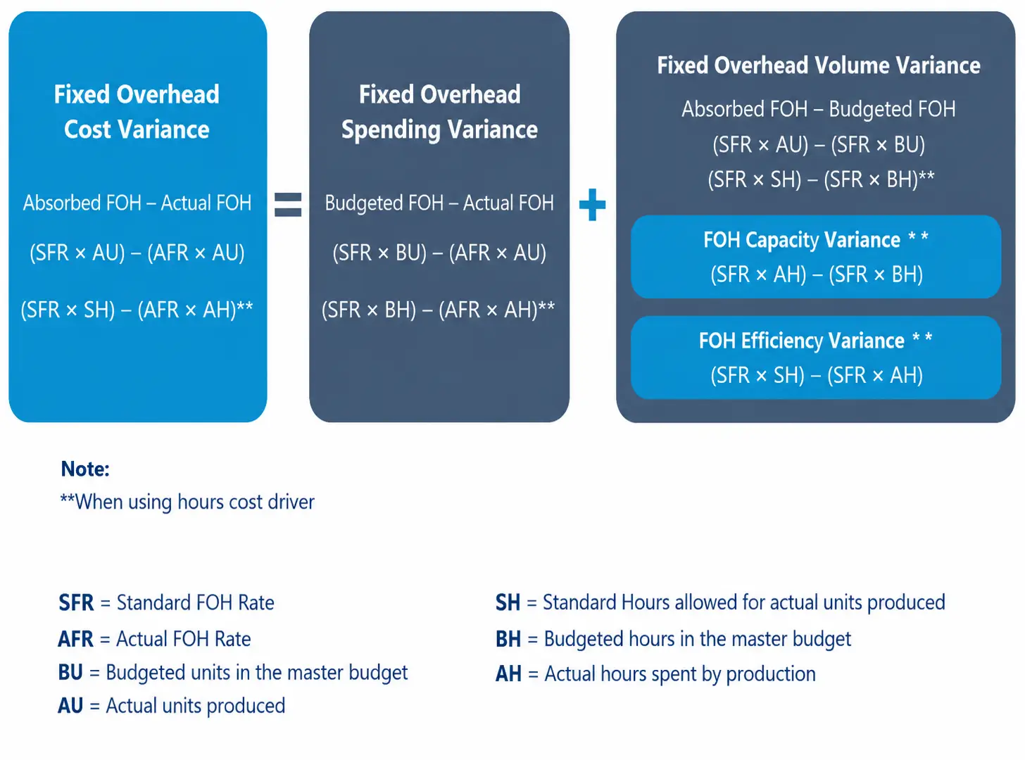
Formulas for fixed overhead cost, spending, volume, capacity, and efficiency variances.
FOH Variances Formulas
Achievable

Production volume variance

The formula for calculating fixed overhead volume variance is:

FOH volume variance=Absorbed FOH−Budgeted FOH

Where:

  • Absorbed FOH is the standard FOH rate × the standard quantity of the cost driver allowed for actual output (i.e., SFR × AU, or SFR × SH)
  • Budgeted FOH is the amount in the master budget

Exam tip: With this orientation, a positive result (absorbed > budgeted) is favorable - actual output beat the budgeted denominator level, so fixed overhead was over-applied. A negative result is unfavorable (under-applied). No fixed costs are actually saved or overspent; the variance only measures capacity utilization. A favorable variance can come from overproduction that builds unwanted inventory, so it isn’t automatically good news.

The following formula may also be helpful in case the CMA problem provided different inputs:

FOH volume variance​=(SFR × AU) − (SFR × BU)=(SFR × SH) − (SFR × BH)​

Where, if the cost driver is units produced:

  • SFR is the standard FOH rate. This could be calculated using the master budget.
  • BU are the budgeted units expected to be produced in the master budget.
  • AU are the actual units produced.

Mathematically, since the SFR is constant in the formula, we are computing the effects of the differences between Actual units produced (AU) versus the Budgeted units (BU).

Where, if the cost driver is not units produced:

  • BH are the budgeted hours in the master budget
  • SH are the standard hours allowed for the actual units produced.

Watch out: When the cost driver is not units produced, SH represents the standard hours allowed for actual production, not the Actual hours (AH) incurred. AH is used only when computing the FOH capacity and efficiency variances below.

The table below shows the FOH volume variance for several different production scenarios:

FOH volume variance scenarios
Achievable

The table below verifies the FOH cost variance by summing the spending and volume variances for the same scenarios:

FOH variances summary of the scenario
Achievable

When the cost drivers for the FOH are not the units of production (e.g., machine hours), the fixed overhead (FOH) volume variance can be further analyzed through its two subcategories:

  1. Capacity variance
  2. Efficiency variance

Together, these subcategories provide deeper insights into whether variances arise from the under- or over-utilization of available production capacity or inefficiencies in the actual output relative to standard expectations.

FOH capacity variance

The FOH capacity variance is a component of the volume variance and it calculates the difference of the actual hours incurred by production versus the budgeted hours from the master budget, applying the standard FOH rate. Mathematically:

FOH capacity variance=(SFR × AH) − (SFR × BH)

Where:

  • SFR is the standard FOH rate. This could be calculated using the master budget.
  • BH are the budgeted (denominator-level) hours in the master budget.
  • AH are the actual hours incurred by production.

The portion of the formula (SFR × BH) refers to the Budgeted FOH in the master budget.

Since the SFR is constant in the formula, we are computing the effects of the differences between Actual hours incurred by production (AH) versus the Budgeted hours (BH).

When actual hours exceed budgeted hours, the variance is favorable because it indicates better utilization of production capacity. This means fixed overhead costs, which remain constant regardless of activity, are spread over more hours, effectively reducing the cost per unit of output and improving resource efficiency. Conversely, fewer actual hours result in an unfavorable variance, as capacity is underutilized, leading to higher fixed costs per unit.

FOH efficiency variance

The FOH efficiency variance is a component of the volume variance and it calculates the difference between the standard hours allowed for the actual units produced versus the actual hours incurred by production:

FOH efficiency variance=(SFR × SH) − (SFR × AH)

Where:

  • SFR is the standard FOH rate. This could be calculated using the master budget.
  • SH are the standard hours allowed for the actual units produced.
  • AH are the actual hours incurred by production.

The portion of the formula (SFR × SH) refers to the Absorbed FOH.

Since the SFR is constant in the formula, we are computing the effects of the differences between Standard hours allowed for actual production (SH) versus the Actual hours incurred by production (AH).

When standard hours exceed actual hours, the variance is favorable, as it indicates efficient use of labor or resources (i.e., less time was required to produce the expected output). Conversely, when actual hours exceed standard hours, the variance is unfavorable, as it suggests inefficiencies in production, requiring more time than expected to achieve the same level of output. This variance highlights how effectively production resources are utilized relative to expectations.

Example: FOH volume, capacity, and efficiency variances

Budgeted FOH is $100,000 based on 10,000 budgeted hours (BH), so the standard FOH rate (SFR) is $100,000 ÷ 10,000 = $10 per hour. For the period, actual production earned 9,000 standard hours (SH), and the actual hours incurred (AH) were 9,500.

  • FOH volume variance: ($10×9,000)−($10×10,000)=$90,000−$100,000=−$10,000 (unfavorable)
  • FOH capacity variance: ($10×9,500)−($10×10,000)=$95,000−$100,000=−$5,000 (unfavorable)
  • FOH efficiency variance: ($10×9,000)−($10×9,500)=$90,000−$95,000=−$5,000 (unfavorable)

Check: the capacity and efficiency variances add up to the volume variance: −$5,000+(−$5,000)=−$10,000.

Answer: The $10,000 unfavorable volume variance splits into a $5,000 unfavorable capacity variance (fewer actual hours than budgeted) and a $5,000 unfavorable efficiency variance (more actual hours used than standard allowed).

FOH volume variance

  • Formula: FOH volume variance=Absorbed FOH−Budgeted FOH, where Absorbed FOH = SFR × AU (or SFR × SH)
  • Alternate form: (SFR×AU)−(SFR×BU) or (SFR×SH)−(SFR×BH)
  • Positive (absorbed > budgeted) = favorable (over-applied FOH); negative = unfavorable (under-applied)
  • Measures capacity utilization only, not actual cost savings/overspending
  • Favorable variance can signal overproduction/excess inventory, not necessarily good
  • SH = standard hours allowed for actual output (not actual hours incurred, AH)

FOH capacity variance

  • Formula: FOH capacity variance=(SFR×AH)−(SFR×BH)
  • Compares actual hours (AH) incurred to budgeted/denominator-level hours (BH)
  • AH > BH → favorable (better capacity utilization, fixed costs spread over more hours)
  • AH < BH → unfavorable (capacity underutilized, higher fixed cost per unit)

FOH efficiency variance

  • Formula: FOH efficiency variance=(SFR×SH)−(SFR×AH)
  • Compares standard hours allowed for actual output (SH) to actual hours incurred (AH)
  • SH > AH → favorable (efficient use of time/resources)
  • SH < AH → unfavorable (took longer than standard, inefficient production)

Relationship & verification

  • Capacity variance + Efficiency variance = Volume variance (check calculation)
  • SFR (standard FOH rate) stays constant across all three formulas; only the hour/unit inputs change
  • Example: $10,000 unfavorable volume variance = $5,000 unfavorable capacity + $5,000 unfavorable efficiency

Sign up for free to take 10 quiz questions on this topic

Previous
Next  | 3.1.4.6.4 FOH cost variance scenario
All rights reserved ©2016 - 2026 Achievable, Inc.

Production volume variance

Production volume variance

The formula for calculating fixed overhead volume variance is:

FOH volume variance=Absorbed FOH−Budgeted FOH

Where:

  • Absorbed FOH is the standard FOH rate × the standard quantity of the cost driver allowed for actual output (i.e., SFR × AU, or SFR × SH)
  • Budgeted FOH is the amount in the master budget

Exam tip: With this orientation, a positive result (absorbed > budgeted) is favorable - actual output beat the budgeted denominator level, so fixed overhead was over-applied. A negative result is unfavorable (under-applied). No fixed costs are actually saved or overspent; the variance only measures capacity utilization. A favorable variance can come from overproduction that builds unwanted inventory, so it isn’t automatically good news.

The following formula may also be helpful in case the CMA problem provided different inputs:

FOH volume variance​=(SFR × AU) − (SFR × BU)=(SFR × SH) − (SFR × BH)​

Where, if the cost driver is units produced:

  • SFR is the standard FOH rate. This could be calculated using the master budget.
  • BU are the budgeted units expected to be produced in the master budget.
  • AU are the actual units produced.

Mathematically, since the SFR is constant in the formula, we are computing the effects of the differences between Actual units produced (AU) versus the Budgeted units (BU).

Where, if the cost driver is not units produced:

  • BH are the budgeted hours in the master budget
  • SH are the standard hours allowed for the actual units produced.

Watch out: When the cost driver is not units produced, SH represents the standard hours allowed for actual production, not the Actual hours (AH) incurred. AH is used only when computing the FOH capacity and efficiency variances below.

The table below shows the FOH volume variance for several different production scenarios:

The table below verifies the FOH cost variance by summing the spending and volume variances for the same scenarios:

When the cost drivers for the FOH are not the units of production (e.g., machine hours), the fixed overhead (FOH) volume variance can be further analyzed through its two subcategories:

  1. Capacity variance
  2. Efficiency variance

Together, these subcategories provide deeper insights into whether variances arise from the under- or over-utilization of available production capacity or inefficiencies in the actual output relative to standard expectations.

FOH capacity variance

The FOH capacity variance is a component of the volume variance and it calculates the difference of the actual hours incurred by production versus the budgeted hours from the master budget, applying the standard FOH rate. Mathematically:

FOH capacity variance=(SFR × AH) − (SFR × BH)

Where:

  • SFR is the standard FOH rate. This could be calculated using the master budget.
  • BH are the budgeted (denominator-level) hours in the master budget.
  • AH are the actual hours incurred by production.

The portion of the formula (SFR × BH) refers to the Budgeted FOH in the master budget.

Since the SFR is constant in the formula, we are computing the effects of the differences between Actual hours incurred by production (AH) versus the Budgeted hours (BH).

When actual hours exceed budgeted hours, the variance is favorable because it indicates better utilization of production capacity. This means fixed overhead costs, which remain constant regardless of activity, are spread over more hours, effectively reducing the cost per unit of output and improving resource efficiency. Conversely, fewer actual hours result in an unfavorable variance, as capacity is underutilized, leading to higher fixed costs per unit.

FOH efficiency variance

The FOH efficiency variance is a component of the volume variance and it calculates the difference between the standard hours allowed for the actual units produced versus the actual hours incurred by production:

FOH efficiency variance=(SFR × SH) − (SFR × AH)

Where:

  • SFR is the standard FOH rate. This could be calculated using the master budget.
  • SH are the standard hours allowed for the actual units produced.
  • AH are the actual hours incurred by production.

The portion of the formula (SFR × SH) refers to the Absorbed FOH.

Since the SFR is constant in the formula, we are computing the effects of the differences between Standard hours allowed for actual production (SH) versus the Actual hours incurred by production (AH).

When standard hours exceed actual hours, the variance is favorable, as it indicates efficient use of labor or resources (i.e., less time was required to produce the expected output). Conversely, when actual hours exceed standard hours, the variance is unfavorable, as it suggests inefficiencies in production, requiring more time than expected to achieve the same level of output. This variance highlights how effectively production resources are utilized relative to expectations.

Example: FOH volume, capacity, and efficiency variances

Budgeted FOH is $100,000 based on 10,000 budgeted hours (BH), so the standard FOH rate (SFR) is $100,000 ÷ 10,000 = $10 per hour. For the period, actual production earned 9,000 standard hours (SH), and the actual hours incurred (AH) were 9,500.

  • FOH volume variance: ($10×9,000)−($10×10,000)=$90,000−$100,000=−$10,000 (unfavorable)
  • FOH capacity variance: ($10×9,500)−($10×10,000)=$95,000−$100,000=−$5,000 (unfavorable)
  • FOH efficiency variance: ($10×9,000)−($10×9,500)=$90,000−$95,000=−$5,000 (unfavorable)

Check: the capacity and efficiency variances add up to the volume variance: −$5,000+(−$5,000)=−$10,000.

Answer: The $10,000 unfavorable volume variance splits into a $5,000 unfavorable capacity variance (fewer actual hours than budgeted) and a $5,000 unfavorable efficiency variance (more actual hours used than standard allowed).

Key points

FOH volume variance

  • Formula: FOH volume variance=Absorbed FOH−Budgeted FOH, where Absorbed FOH = SFR × AU (or SFR × SH)
  • Alternate form: (SFR×AU)−(SFR×BU) or (SFR×SH)−(SFR×BH)
  • Positive (absorbed > budgeted) = favorable (over-applied FOH); negative = unfavorable (under-applied)
  • Measures capacity utilization only, not actual cost savings/overspending
  • Favorable variance can signal overproduction/excess inventory, not necessarily good
  • SH = standard hours allowed for actual output (not actual hours incurred, AH)

FOH capacity variance

  • Formula: FOH capacity variance=(SFR×AH)−(SFR×BH)
  • Compares actual hours (AH) incurred to budgeted/denominator-level hours (BH)
  • AH > BH → favorable (better capacity utilization, fixed costs spread over more hours)
  • AH < BH → unfavorable (capacity underutilized, higher fixed cost per unit)

FOH efficiency variance

  • Formula: FOH efficiency variance=(SFR×SH)−(SFR×AH)
  • Compares standard hours allowed for actual output (SH) to actual hours incurred (AH)
  • SH > AH → favorable (efficient use of time/resources)
  • SH < AH → unfavorable (took longer than standard, inefficient production)

Relationship & verification

  • Capacity variance + Efficiency variance = Volume variance (check calculation)
  • SFR (standard FOH rate) stays constant across all three formulas; only the hour/unit inputs change
  • Example: $10,000 unfavorable volume variance = $5,000 unfavorable capacity + $5,000 unfavorable efficiency

More from Fixed overhead (FOH) cost variance

  • Overview of FOH cost variance formula
  • FOH spending variance
  • FOH cost variance scenario