In this chapter, you’ll learn the fundamentals of forecasting used by different businesses. You’ve already explored one forecasting method (the linear equation). Here, the focus is on the time series approach.

Time series model

A time series model is one of the most widely used approaches to forecasting. It breaks historical data into four components:

Trend
Seasonal
Cyclical
Residual

Trend

Some economists refer to the trend as “time” because it captures the overall direction of the data over time. For example, if you’re forecasting sales for a product, the trend might be:

declining
flat
rising

Below are examples of trendlines.

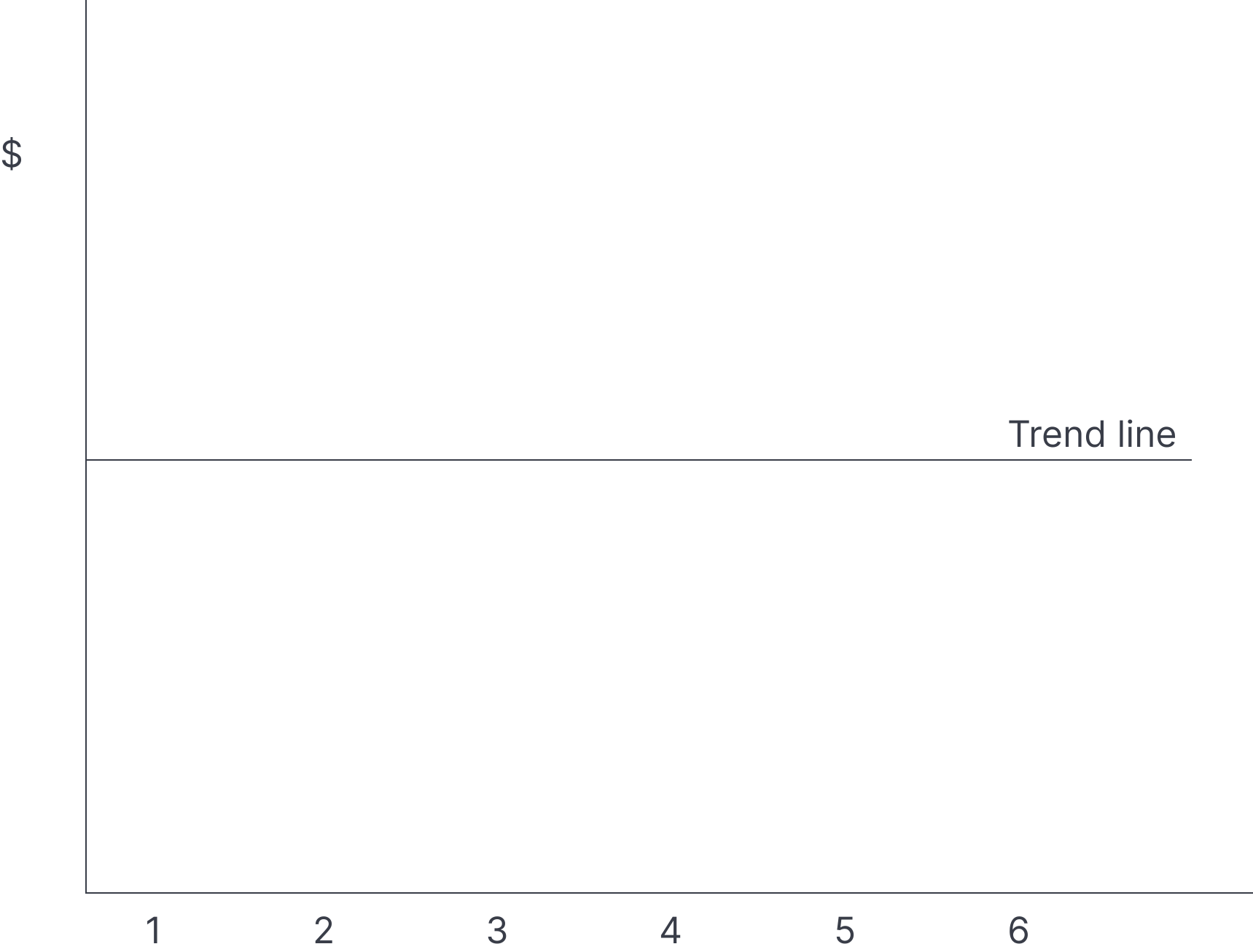
A flat moving trendline, showing neither increase or decrease in results being measured — The flat trendline

The example above shows a flat trend. The overall movement (sales, production, and so on) is steady — neither increasing nor decreasing.

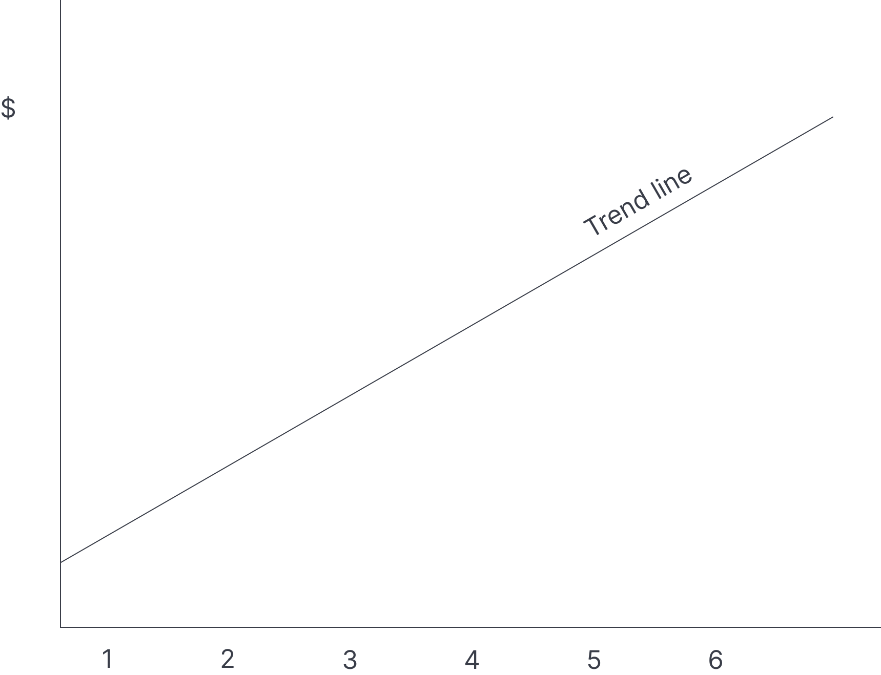
An upward moving trendline, showing increase in results being measured — The uphill trendline

The example above shows an upward (rising) trend. The variable being forecast increases from period to period.

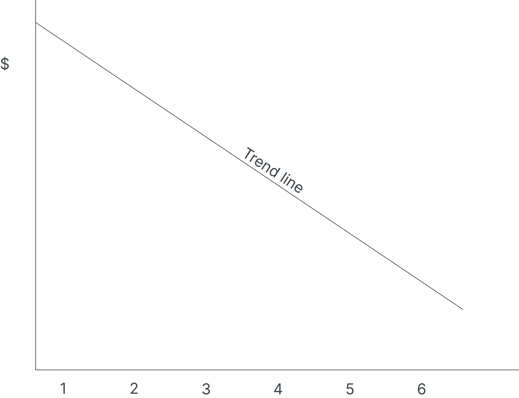
A downward moving trendline, showing decline in results being measured — The downhill trendline

The example above shows a declining trend. Sales (or whatever you’re measuring) decrease over time.

Seasonal variation

Seasonal variation is the repeating up-and-down movement around the trendline. The trendline shows the overall direction, but it doesn’t show the regular short-term patterns that repeat within the year (or within another fixed cycle).

For example, if you sell ice cream, you might see two clear seasons:

winter: sales are lower (below trend)
summer: sales are higher (above trend)

Seasonal variation can occur around any trend: flat, rising, or declining.

Below are examples of seasonal variation.

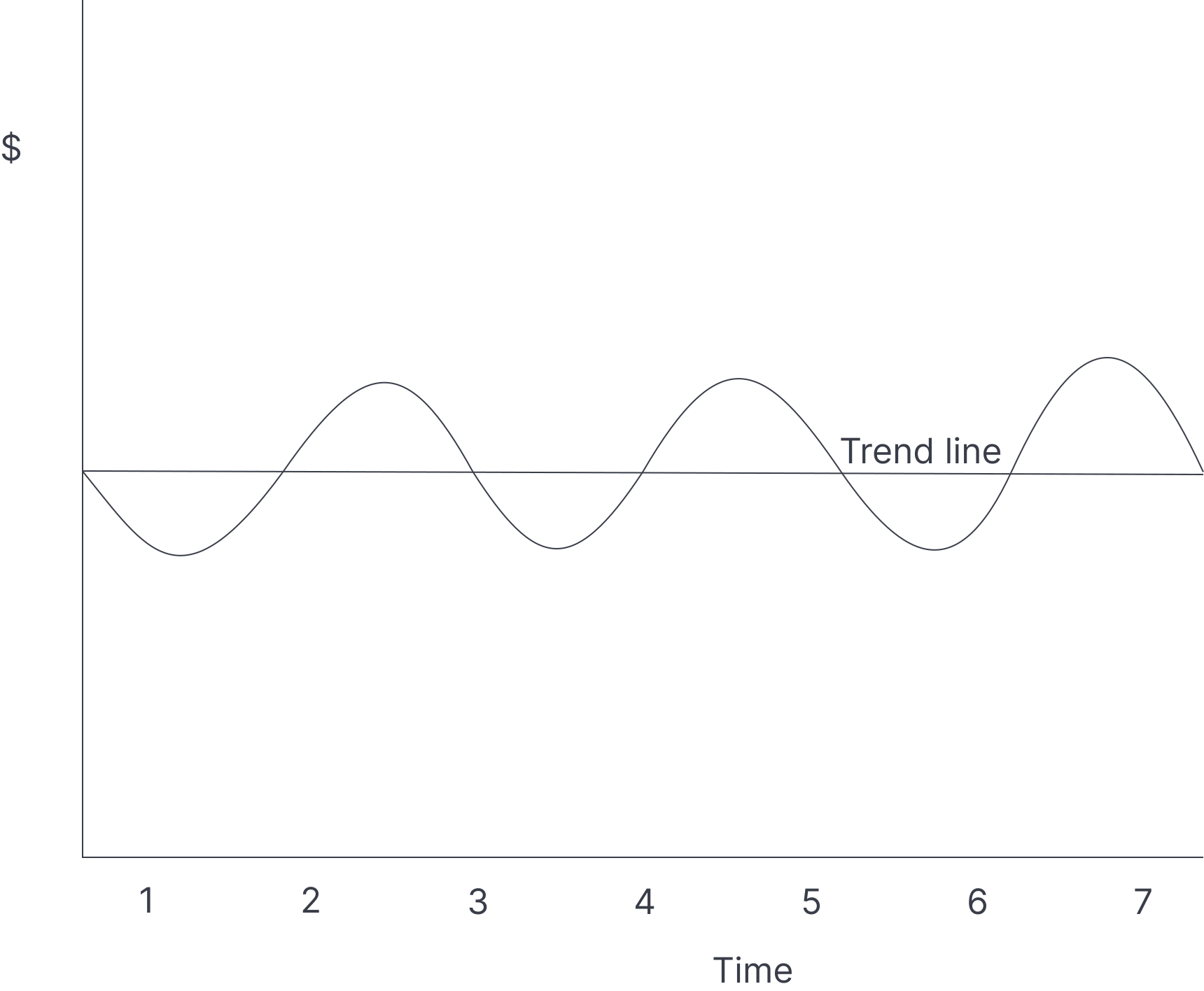
A graph showing the seasonal variation on a flat trendline, showing the seasonal variation is going up and down but maintaining the same average — Seasonal variation on flat trendline

In the graph above, the seasonal pattern moves up and down, but the average level stays the same. That’s why the overall trend remains flat.

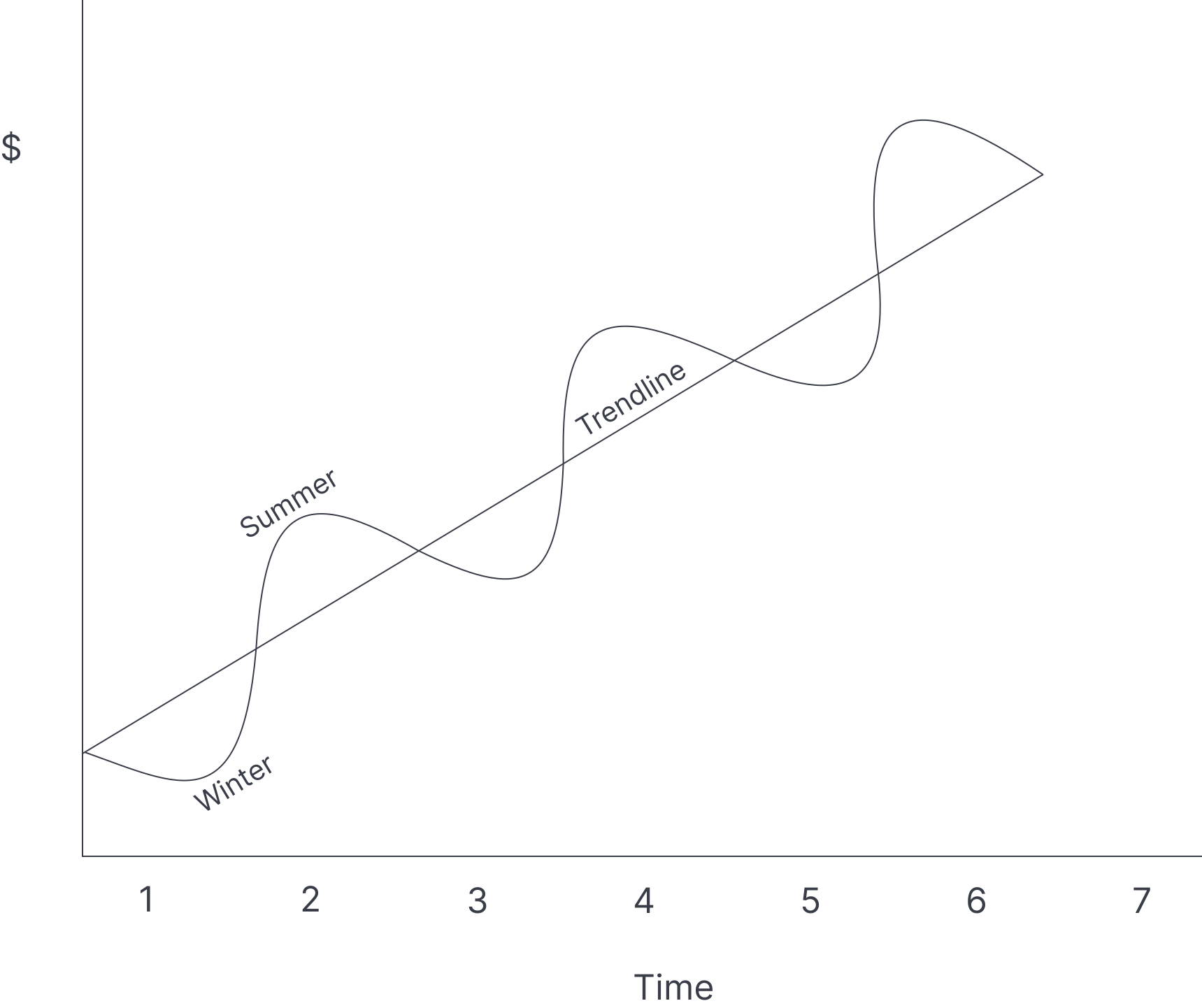
A graph showing the seasonal variation moving upward, which shows that the seasonal variation is increasing along with the trend — Seasonal variation on an uphill trendline

In the graph above, the trend rises over time, and the seasonal pattern still moves above and below the trend. That means:

in some periods, sales are higher than the trend
in other periods, sales are lower than the trend

(We’re using sales as an example, but the same idea applies to any variable you forecast.)

Cyclical variations

Cyclical variation comes from broader economic or business cycles. For example, in early 2020 during COVID, South Africa recorded very low car sales (just below 600 cars) compared with the normal average of about 4,000 cars per month at that time. During the same period, streaming companies such as Netflix, Disney, and Amazon Prime saw subscriptions rise to record levels.

Cyclical effects can be:

positive
negative

Unlike seasonal variation, cyclical variation is difficult to predict. Because of that, it’s often ignored in calculations (as you’ll see in the formulas later). However:

if the examiner clearly gives you a cyclical component, you must use it
if the cyclical component is missing and the question expects you to find it, you must calculate it

Key example

At the time this text was written, several wars were taking place (for example, the war between Russia and Ukraine). These events affected resource prices, especially in the energy sector worldwide. Below is a list of companies that were heavily impacted by the Russia-Ukraine war, according to Wikipedia.

Company	Industry	Origin	Suspended services	Start date
3M	Conglomerate	United States	all operations in Russia	2022
Accenture	Consulting	Ireland	closing business in Russia	2022
Activision Blizzard	Video game	United States	all sales in Russia	2022
Advanced Micro Devices	Semiconductor company	United States	chip sales to Russia	2022
Adidas	Clothing	Germany	partnership with Russian Football Union	2 March 2022

Residual components

Residual components are random, unexpected effects. For example:

a business building burns down
high-value stock is stolen

Like cyclical variation, residual effects are usually ignored in time series analysis because they’re difficult to predict.

Formulas

There are two methods of handling a time series question:

the additive model
the multiplicative model

The examiner will indicate which method to use, so you don’t need to guess in an exam question. Your job is to understand both methods.

The formula for the additive model is:

$Y = T + S + C + R$

which is simplified to:

$Y = T + S$

Under this model, all components are expressed in monetary terms, meaning the decision maker works with real figures throughout. However, because all values are in monetary terms, the figures can be easily distorted by inflation over time. This is why most economists recommend the multiplicative model.

The formula for the multiplicative model is:

$Y = T \times S \times C \times R$

which is simplified to:

$Y = T \times S$

Under this model, only the trend is expressed in monetary terms. The remaining components are expressed as multiplying factors — for example, $0.98$ , $1.15$ , $0.88$ , and so on. This makes the model less susceptible to distortion by inflation.

From now on we will focus on the calculation of two components: the trendline and the seasonal variations.

Time series model

Breaks historical data into four components: trend, seasonal, cyclical, residual
Widely used for business forecasting

Trend

Captures overall direction over time (rising, flat, declining)
Shown by trendlines (upward, flat, downward)

Seasonal variation

Repeating short-term patterns within a fixed cycle (e.g., year)
Moves above and below the trendline
Can occur with any trend direction

Cyclical variations

Caused by broader economic or business cycles (e.g., recessions, wars)
Effects can be positive or negative
Difficult to predict; often ignored unless specified

Residual components

Random, unexpected effects (e.g., disasters, theft)
Usually ignored in analysis due to unpredictability

Formulas

Additive model: $Y = T + S + C + R$ (often simplified to $Y = T + S$ )
- All components in monetary terms; can be distorted by inflation
Multiplicative model: $Y = T \times S \times C \times R$ (often simplified to $Y = T \times S$ )
- Only trend in monetary terms; less affected by inflation
Examiner will specify which model to use

Next | 11.2 Trendline calculation methods

Fundamentals of time series model

Time series model

A time series model is one of the most widely used approaches to forecasting. It breaks historical data into four components:

Trend
Seasonal
Cyclical
Residual

Trend

Some economists refer to the trend as “time” because it captures the overall direction of the data over time. For example, if you’re forecasting sales for a product, the trend might be:

declining
flat
rising

Below are examples of trendlines.

The example above shows a flat trend. The overall movement (sales, production, and so on) is steady — neither increasing nor decreasing.

The example above shows an upward (rising) trend. The variable being forecast increases from period to period.

The example above shows a declining trend. Sales (or whatever you’re measuring) decrease over time.

Seasonal variation

For example, if you sell ice cream, you might see two clear seasons:

winter: sales are lower (below trend)
summer: sales are higher (above trend)

Seasonal variation can occur around any trend: flat, rising, or declining.

Below are examples of seasonal variation.

In the graph above, the seasonal pattern moves up and down, but the average level stays the same. That’s why the overall trend remains flat.

In the graph above, the trend rises over time, and the seasonal pattern still moves above and below the trend. That means:

in some periods, sales are higher than the trend
in other periods, sales are lower than the trend

(We’re using sales as an example, but the same idea applies to any variable you forecast.)

Cyclical variations

Cyclical effects can be:

positive
negative

Unlike seasonal variation, cyclical variation is difficult to predict. Because of that, it’s often ignored in calculations (as you’ll see in the formulas later). However:

if the examiner clearly gives you a cyclical component, you must use it
if the cyclical component is missing and the question expects you to find it, you must calculate it

Key example

Company	Industry	Origin	Suspended services	Start date
3M	Conglomerate	United States	all operations in Russia	2022
Accenture	Consulting	Ireland	closing business in Russia	2022
Activision Blizzard	Video game	United States	all sales in Russia	2022
Advanced Micro Devices	Semiconductor company	United States	chip sales to Russia	2022
Adidas	Clothing	Germany	partnership with Russian Football Union	2 March 2022

Residual components

Residual components are random, unexpected effects. For example:

a business building burns down
high-value stock is stolen

Like cyclical variation, residual effects are usually ignored in time series analysis because they’re difficult to predict.

Formulas

There are two methods of handling a time series question:

the additive model
the multiplicative model

The examiner will indicate which method to use, so you don’t need to guess in an exam question. Your job is to understand both methods.

The formula for the additive model is:

$Y = T + S + C + R$

which is simplified to:

$Y = T + S$

The formula for the multiplicative model is:

$Y = T \times S \times C \times R$

which is simplified to:

$Y = T \times S$

From now on we will focus on the calculation of two components: the trendline and the seasonal variations.

CGMA BA1

11. Time series model

Our CGMA course is currently in development and is a work-in-progress.