Averaging data

Arithmetic mean

The graphs and charts we’ve used so far are useful for visualizing data, but you also need numerical measures to interpret what the data is saying. One common measure is the arithmetic mean (often just called the mean). It’s the “average” value of a data set.

You’ll see how to calculate the mean for:

• simple (ungrouped) data
• frequency data
• grouped data

Let’s use data from example 2 to calculate the mean.

Sales
Content creation	100000
Lecturing	60000
Textbook sales	40000
Advisory	15000
Total	215000

To find the mean, divide the total by the number of values.

The formula for calculating mean as follows: (Brenden will put up the necessary sign of the formula)

$$\frac{215000}{4}=53750$$

This means the average sales per segment is $53750.

The mean can be helpful, for example, when you want a single number that summarizes typical sales across segments. At the same time, notice a limitation: the mean doesn’t have to be one of the values in the data set. Here, $53750 isn’t in the list, and it sits above two of the four values ($15000 and $40000). That’s why the mean is often used alongside other measures.

Later in the text we will consider other methods that can be used alongside the arithmetic mean to extract meaning from a data set.

What if you are asked to calculate arithmetic mean from frequency? Let’s look at one example.

KTA has taken interest in the attendance record of its students as a way of improving the pass rates. It has taken data from the register of the previous month (20-day school month)

3	3	1	1	2
0	0	0	0	0
5	4	6	8	1
3	5	5	4	4

The frequency table will look as follows:

Number of absent days	Frequency
0	5
1	3
2	1
3	3
4	3
5	3
6	1
7	1
Grand total	20

Now, let’s look at the calculations.

To find the mean from a frequency table:

• multiply each value $X$ by its frequency $Y$
• add those products to get the total of $X(Y)$
• divide by the total frequency

X (number of absent days)	Y (Frequency)	X(Y)
0	5	0
1	3	3
2	1	2
3	3	9
4	3	12
5	3	15
6	1	6
7	1	7
Grand total	20	54

Then next, let’s get into our final calculations.

$$\frac{54}{20}=2.7$$

According to our calculations, the average number of days students missed classes was 2,7 days. To the nearest day, that’s 3 days.

How about grouped data?

Let’s look at an example again to gain some understanding of the calculation. We will use some information from example 1. Keep in mind that the formula will be the same as for the frequency, the only difference is that for the $X$ values we use the midpoints of each class.

Time	tally
50 to below 55	4
55 to below 60	7
60 to below 65	4
65 to below 70	9

The above is the original data, now let’s insert midpoints on the x values.

X (midpoint)	Frequency	F(X)
52,5	4	210
57,5	7	402,5
62,5	4	250
67,5	9	607,5
Total	24	1470

Using the previous formula, the arithmetic mean will be:

$$\frac{1470}{24}=61.25$$

We will now consider another form of average.

Median

The median is the middle value in a data set when the values are arranged in order.

We will learn how to calculate mode on simple data, frequency and grouped data, as we have done when we were calculating arithmetic mean.

Let’s use some information from example 2 as shown below:

Sales
Content creation	100000
Lecturing	60000
Textbook sales	40000
Advisory	15000
Total	215000

First, arrange the data in ascending order: $15000, $40000, $60000, $100000.

Because there are 4 values (an even number), there isn’t a single middle value. The two middle values are $40000 and $60000, so we add them and divide by 2:

• $40000 + $60000 = $100000
• $100000÷2=$ 50000

So the median is $50 000.

Please it’s not compulsory to add the middle numbers and divide by 2, we do this when there is no obvious middle number.

How do we calculate median from frequency?

Let’s bring an example we have looked at before. We will use information from example 1, which is as follows:

Time	Frequency
50	0
55	4
60	11
65	15
70	24

The formula is as follows:

$$\frac{n+1}{2}$$

In our case:

$$\frac{24+1}{2}=12.5$$

What if you are given grouped data to deal with?

Let us use example 1 data to solve the issue.

Time	tally	Freq
50 to below 55	4	4
55 to below 60	7	11
60 to below 65	4	15
65 to below 70	9	24

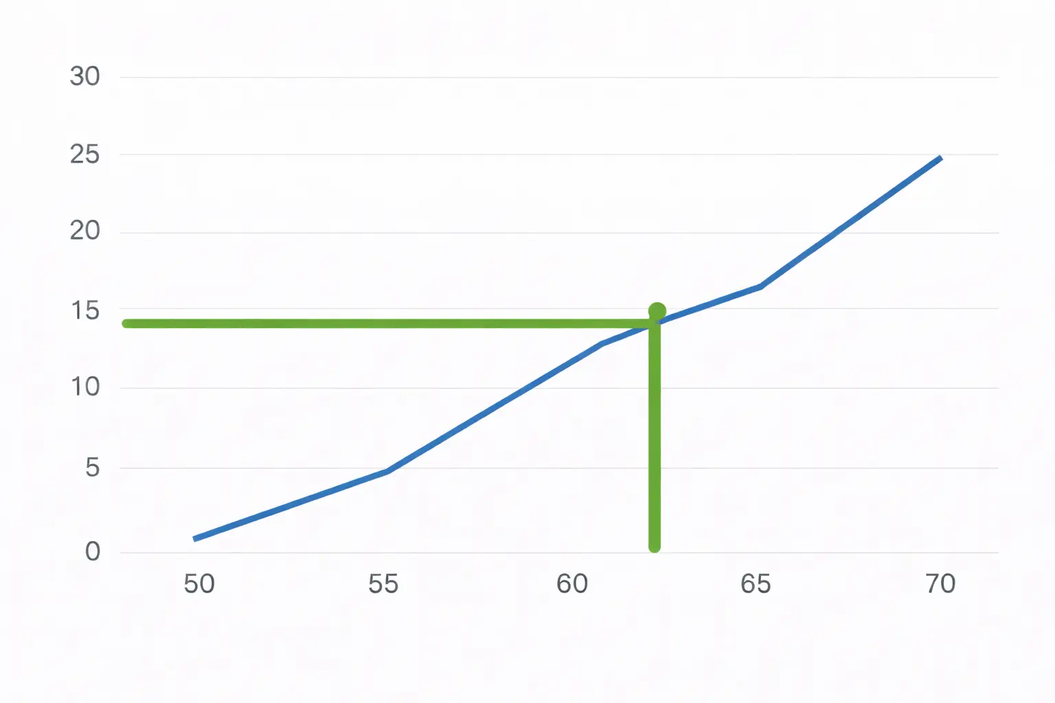
Our total cumulative frequency is 24, so half of that is 12. To estimate the median from the cumulative curve:

• locate 12 on the y axis
• draw a horizontal line until it touches the curve
• from that point, drop a vertical line down to the x axis

That x-value is the median. In our case, as indicated by the graph, it is approximately 61 mins.

Mode

The mode is the value (or class) that occurs most often.

• In simple or frequency data, it’s the number with the highest frequency.
• In grouped data, it’s the class interval with the highest frequency (or tally).

Let’s use some previous examples.

Time	tally
50 to below 55	4
55 to below 60	7
60 to below 65	4
65 to below 70	9

In the above, the mode is the class with the highest frequency: 65 to below 70 (frequency 9).

Number of absent days	Frequency
0	5
1	3
2	1
3	3
4	3
5	3
6	1
7	1
Grand total	20

From the above data mode is 3 since it is appearing the most hence the highest frequency.