Graphs & curve sketching
To analyze a function, you need to connect what you see on the graph of to what its derivatives say about slope and concavity. On the AP exam, many multiple-choice questions on this topic focus more on reasoning from these connections than on computing exact values.
Connecting and
Recall from the previous sections:
The 1st derivative tells you where the function is going (slope of the tangent line).
| Condition | What it means for |
|---|---|
| Increasing | |
| Decreasing | |
| or undefined | Critical point at |
| changes sign at | Relative extremum |
The 2nd derivative tells you about the shape of .
| Condition | What it means for |
|---|---|
| Concave up | |
| Concave down | |
| or undefined and changes sign | Inflection point |
Additionally, because is the derivative of , the same fundamental relationships apply. For example, if , then is increasing.
Example 1: Identifying from
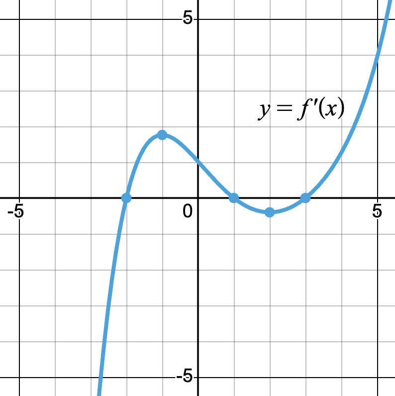
Shown below is the graph of , the derivative of .
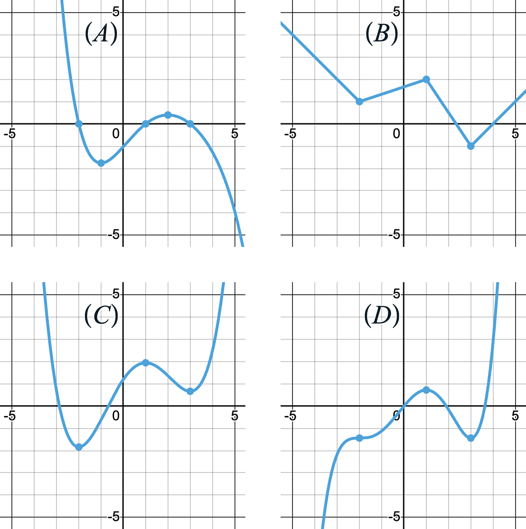
Which one of the 4 graphs below could be the graph of ?
Solution
Step 1: Locate the critical points of .
is a polynomial and therefore defined for all values.
when the graph shown crosses the -axis.
- Occurs at and , which are therefore critical points of .
Step 2: Analyze sign changes of
-
At : changes from negative to positive relative min at .
-
At : changes from positive to negative relative max at .
-
At : changes from negative to positive relative min at .
You may also justify using the 2nd derivative test by reading whether is increasing or decreasing at each critical point:
-
At : is increasing, so relative min
-
At : is decreasing, so relative max
-
At : is increasing, so relative min
Only graphs B and C show extrema in this order, so A and D can be eliminated.
Step 3: Additional identifying information
Notice that graph B consists of straight-line segments with sharp corners at . Since corners are not differentiable, the graph of for choice B would be undefined. However, the given graph of is a polynomial that shows each point to equal .
So graph B can be eliminated, and graph C is the only option.
Example 2: Comparing and
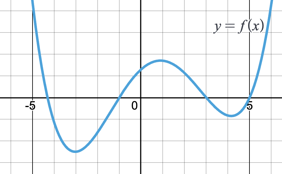
Shown below is the graph of a twice-differentiable function . It has extrema at and and its inflection points occur at and .
At which point is ?
Solution
Answer: (choice D)
Let’s analyze each point:
At :
- (graph is below the -axis).
- (relative min at ).
- Since , this answer choice can be eliminated.
At :
- (graph crosses the -axis)
- ( is increasing).
- Since , this answer choice can also be eliminated.
At :
- (relative max at ).
- (concave down)
- Since , this choice can be eliminated.
At :
- ( is decreasing).
- ( changes concavity at ).
- Since , this is the correct point.
Curve sketching
You may have sketched general shapes of polynomial, rational, exponential, and other functions in Precalculus by finding intercepts and end behavior. Calculus allows you to sketch more accurate graphs by analyzing a function’s behavior.
To sketch the shape of a function:
- Find its domain, intercepts, and asymptotes (if any)
- Find critical points (1st derivative )
- Test intervals for increasing/decreasing behavior of and/or classify extrema
- Find inflection points (2nd derivative )
- Test intervals for concavity of
- Piece it all together
Sketch the graph of
Solution
Step 1: Identify asymptotes, intercepts, and domain
- Vertical asymptotes: and
- Horizontal asymptote:
- -intercepts (when ):
- -intercept (when ):
- Domain: and
Step 2: Critical points
With the quotient rule,
Now identify where or is undefined.
is undefined when and . These are vertical asymptotes where is undefined, so they are not critical points of .
when , which has no real solutions. So has no relative extrema.
Step 3: Increasing and decreasing intervals
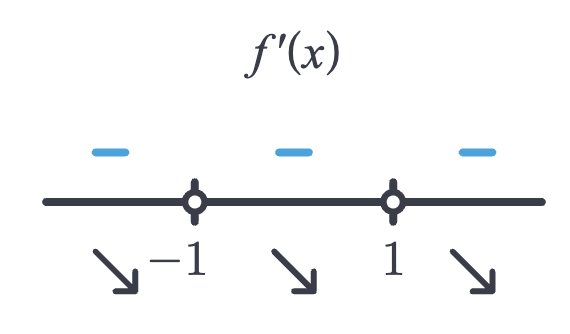
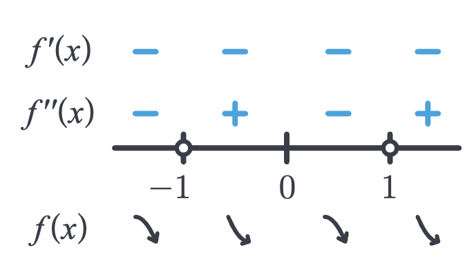
Choose a test point in each interval of the domain (split by the vertical asymptotes at and ) and determine the sign of . Instead of a chart, the signs are depicted as a diagram:
is decreasing on all three intervals of its domain because . When sketching, it often helps to mark where is undefined (open circles at the asymptotes) and to draw arrows showing the direction of decrease.
Step 4: Inflection points
Differentiate to find :
Simplify by factoring in the numerator:
Potential inflection points occur where (and is defined). Here, when only.
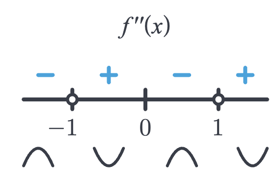
Step 5: Concavity
Test the sign of on each interval. Even though and cannot be inflection points, they still split the domain and should appear on the sign diagram.
As shown, it can be helpful to sketch a small “concave up” or “concave down” curve on each interval to keep the shape straight as you draw the final graph.
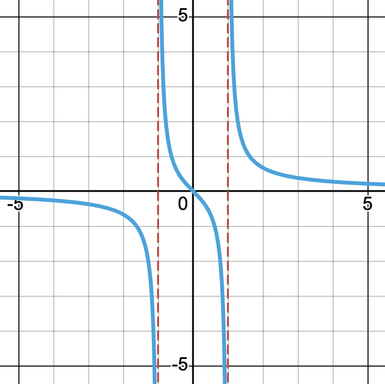
Step 6: Putting it all together
Combine what you know about intercepts, asymptotes, increasing/decreasing behavior, and concavity. For example, on , is decreasing and concave up, and a small curve has been drawn to depict this.
Plot the asymptotes and intercepts, then sketch each branch to match the sign diagrams: