


Inventory systems: periodic
Inventory systems determine when ending inventory and cost of goods sold are measured. That timing ties directly to the cost flow assumptions (FIFO, LIFO, weighted average) covered in the previous chapter.
There are two main systems being used by companies to track their inventories:
- Periodic inventory system, where ending inventory and cost of goods sold are determined and recorded only at the end of the period; and
- Perpetual inventory system, where cost of goods sold is calculated at the time of every individual sale.
A periodic system is simpler and cheaper to maintain, so it suits small businesses with limited resources and a simple inventory tracking process. The trade-off is that it gives no running inventory balance, and losses from theft or damage (shrinkage) cannot be identified separately: they end up in cost of goods sold when the physical count sets ending inventory.
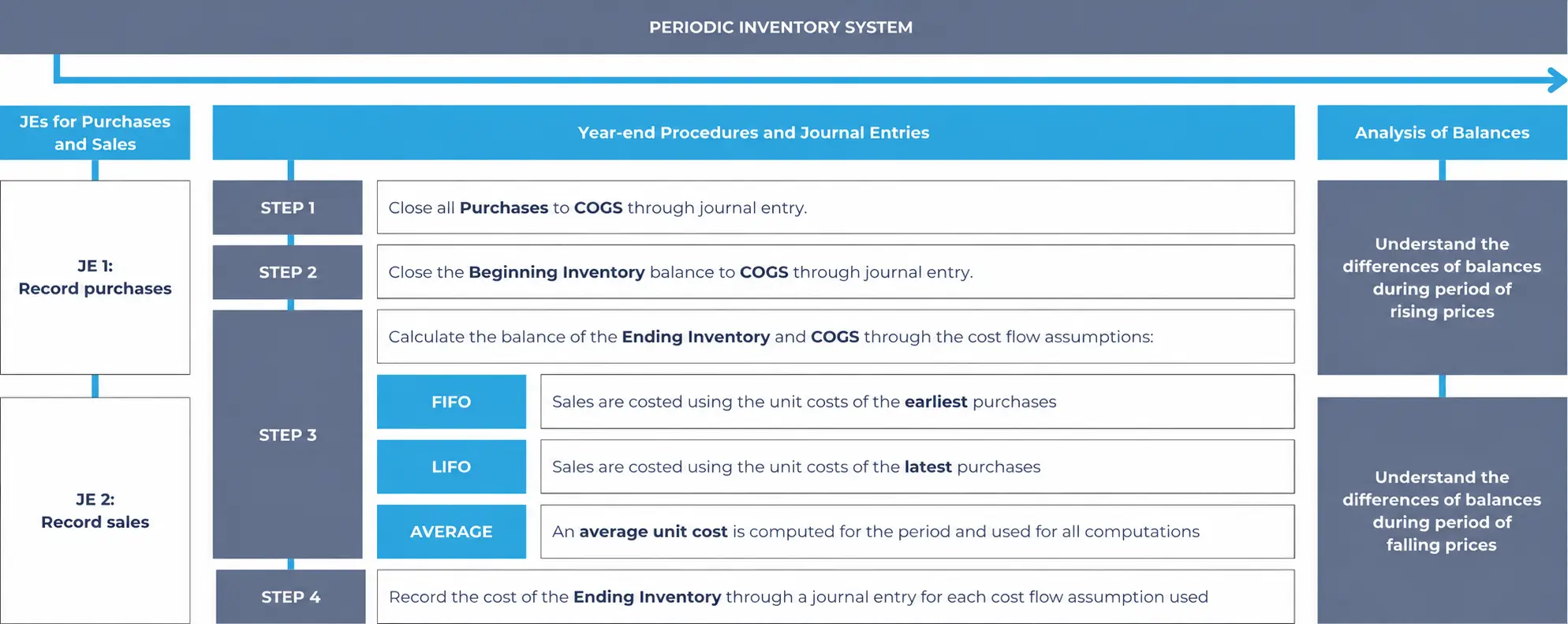
The following concept map for the periodic inventory system could be helpful to navigate through the topic:
Periodic inventory system
The company would traditionally do an inventory count at the end of the period to determine how many units of goods are unsold and then determine the costs of these ending inventory through the cost flow assumptions (FIFO, LIFO, average method, or specific identification). From the cost of the ending inventory, the company can determine the cost of goods sold through a formula.
Details of the steps and journal entries under the periodic inventory system are discussed below. It is good to note that under this system, the balance of the ending inventory and cost of goods sold are not affected by the day-to-day purchase and sale of inventories but are only established during year-end procedures.
Journal entries under the periodic system
JE 1: record purchases under periodic system
Under the periodic inventory system, when inventory is purchased it is recorded in a temporary “Purchases” account in the income statement. The inventory purchased is not recorded in an asset account but in a temporary account.
| Account | Debit | Credit | Financial statement element |
| Purchases | XXX | Expense | |
| Cash or accounts payable | XXX | Asset or liability | |
| To record purchases of inventory | |||
JE 2: record sales under periodic system
Under the periodic inventory system, when inventory is sold, the impact on the inventory account is not recorded. There is only a journal entry to record the sale.
| Account | Debit | Credit | Financial statement element |
| Cash or accounts receivable | XXX | Asset | |
| Sales revenue | XXX | Revenue | |
| To record a sale of inventory | |||
Purchase returns, discounts, and freight-in. Under the periodic system, adjustments to purchases also go to temporary accounts rather than to Inventory:
- A purchase return or allowance is recorded as a debit to accounts payable (or cash) and a credit to Purchase returns and allowances, a contra account to Purchases.
- A discount taken for paying early is credited to Purchase discounts, another contra account to Purchases.
- Transportation costs on incoming goods are debited to Freight-in, which is added to purchases.
Together they give the cost of goods purchased: net purchases (purchases − purchase returns and allowances − purchase discounts) + freight-in. These accounts are closed to COGS along with Purchases in Step 1.
The journal entries above happen all throughout the year and then at the end of the year, the year-end procedures are done.
Year-end procedures under the periodic system
Under the periodic inventory system, you need to follow the following procedures to complete the accounting for ending inventories and cost of goods sold (COGS):
- Step 1: Close all “Purchases” to COGS
- Step 2: Close the beginning balance of inventories to COGS
- Step 3: Determine the cost of ending inventory through the cost flow assumptions and calculate the COGS
- Step 4: Record the cost of the ending inventory
Step 1. Close all “Purchases” to COGS
Under the period inventory system, all purchases accounts (from JE 1 above) are closed to another expense account called “cost of goods sold” or COGS.
The COGS is presented in the income statement as an expense netted against the revenue accounts to arrive at the gross profit.
| Account | Debit | Credit | Financial statement element |
| Cost of goods sold | XXX | Expense | |
| Purchases | XXX | Expense | |
| To close the ending balance of the purchases accounts to COGS | |||
After this journal entry, the balance of “Purchases” account in the income statement is nil.
Step 2. Close beginning balance of inventories to COGS
Under the periodic inventory system, the balance of the “inventory” account in the balance sheet remains unchanged from the previous period. Effectively the ending inventory of the previous period becomes the beginning inventory of the current period.
You need to close the balance of the beginning inventory to the cost of goods sold at the end of the current period to reduce the balance of the inventory account to nil. This is important so that you can now establish the new ending inventory balance in the next step.
| Account | Debit | Credit | Financial statement element |
| Cost of goods sold | XXX | Expense | |
| Inventory | XXX | Asset | |
| To close the beginning balance of inventory to COGS | |||
Inventory has a normal balance of debit. We credit it to reduce the balance to nil. After this journal entry, the balance of the inventory account in the balance sheet resets to zero.
Step 3. Determine the cost of ending inventory through the cost flow assumptions and calculate the COGS
After the previous step, the “inventory” account in the balance sheet is nil.
The next step is to determine the new inventory balance through cost flow assumptions (FIFO, LIFO or average). The amount we will determine becomes the ending inventory for the current period and the beginning inventory for the next period.
In this step, we will only discuss the determination of the cost through the cost flow assumptions and then the journal entry will be discussed in Step 4.
Example: April inventory movements
Below is the summary of inventory movements for the month of April (a period of rising prices) for Achievable:
Date Nature Units Cost Total Apr 1 Beginning inventory 500 $ 2.0 $ 1,000 Apr 2 Purchase 1,000 $ 2.5 $ 2,500 Apr 5 Purchase 1,000 $ 3.0 $ 3,000 Apr 9 Sale (Per unit: 7.00) (800) Apr 15 Purchase 1,500 4.0 $ 6,000 Apr 29 Sale (Per unit: 8.00) (1,200) Apr 30 Ending inventory 2,000 12,500 Before you start, notice the total of $ 12,500 coming from the total costs of the beginning inventory and purchases. This is called the “cost of goods available for sale” during April. This cost will be split between the cost of ending inventory (unsold) and the cost of goods sold.
Step 3.1. FIFO assumption:
Under the FIFO assumption, the ending inventory of 2,000 units will be coming from the latest purchases as follows.
| 1,500 units from the Apr 15 purchase at $4.0 ($4.0 x 1,500) | $6,000 |
| 500 units from the Apr 5 purchase at $3.0 ($3.0 x 500) | $1,500 |
| Total cost of 2,000 units of ending inventory | $7,500 |
The April 5 purchase was effectively split into 500 units sold and 500 units unsold. Cost of goods sold is the cost of goods available for sale minus the cost of ending inventory: $ 12,500 − $ 7,500 = $ 5,000.
Step 3.2. LIFO assumption:
Under the LIFO assumption, the ending inventory of 2,000 units will be coming from the beginning inventory and the oldest purchases as follows.
| 500 units from the beginning inventory at $2.0 ($2.0 x 500) | $1,000 |
| 1,000 units from the Apr 2 purchase at $2.5 ($2.5 x 1,000) | $2,500 |
| 500 units from the Apr 5 purchase at $3.0 ($3.0 x 500) | $1,500 |
| Total cost of 2,000 units of ending inventory | $5,000 |
We do not recommend trying to calculate the LIFO cost of goods sold in detail (like in the FIFO method above) under the periodic inventory system. Instead, obtain it by deducting the cost of ending inventory from the cost of goods available for sale: $12,500 − $5,000 = $7,500.
Step 3.3. Average method assumption:
The average method under the periodic system is called the weighted average method because each unit cost is weighted by the number of units available at that cost (cost of goods available for sale ÷ total units available for sale). The resulting single average cost per unit is used for both:
- ending inventory; and
- cost of goods sold.
It is calculated as follows:
| Cost of goods available for sale (CGAS) | $12,500 |
| Divide by:
Total units available for sale (composed of the total beginning inventory + units purchased during the period) |
4,000 units |
| Average cost per unit | $3.125 per unit |
| Cost of ending inventory
(2,000 units × $3.125) |
$6,250 |
| Cost of goods sold
(2,000 units × $3.125) |
$6,250 |
| Cost of goods available for sale | $12,500 |
You can also obtain the cost of goods sold by deducting the cost of ending inventory from the cost of goods available for sale: $12,500 − $6,250 = $6,250.
Step 4. Record the cost of the ending inventory
Once you have ascertained the amount of inventory balance, you can now post the journal entry. Note that we only post the cost of the ending inventory at the end of the period under the periodic system.
This is done through the COGS account because so far it has accumulated both the total purchases (Step 1) and the beginning balance of the inventories (Step 2). This running total of COGS after Step 2 equals the cost of goods available for sale.
We need to remove the cost of unsold goods (determined in Step 3) from this running total to arrive at the actual cost of goods sold. The journal entry follows the same pattern regardless of the cost flow assumption used - only the dollar amount changes:
| Account | Debit | Credit | Financial statement element |
| Inventory | XXX | Asset | |
| Cost of goods sold | XXX | Expense | |
| To record the ending inventory | |||
Using the amounts from Step 3, the amount (XXX) recorded is:
- FIFO: $7,500 (see Step 3.1)
- LIFO: $5,000 (see Step 3.2)
- Weighted average: $6,250 (see Step 3.3)
Analysis of the ending balances under the periodic system
This section analyzes the balances after all year-end journal entries have been posted, and how they are presented on the income statement.
Using the same example introduced in Step 3, below is a summary of the ending inventory, sales, cost of goods sold, and gross profit under all cost flow assumptions. Recall that April is a period of rising prices for the company.
| Units | FIFO | LIFO | Weighted ave. | |
| Balance sheet: | ||||
| Ending inventory | 2,000 | $7,500 | $5,000 | $6,250 |
| Income statement: | ||||
| Sales | 2,000 | $15,200 | $15,200 | $15,200 |
| Cost of goods sold | 2,000 | ($5,000) | ($7,500) | ($6,250) |
| Gross profit | $10,200 | $7,700 | $8,950 |
The amount of sales is the total sales (Apr 9 and Apr 29) from the example in Step 3.
In a period of rising prices, the example illustrates the following:
- FIFO method has the highest gross profit because the cost of goods sold are based on the lower priced inventory items of the old purchases
- Consequently, LIFO has the highest cost of goods sold and the lowest gross profit
- FIFO has the higher cost of ending inventory in the balance sheet because these are based on the higher priced most current purchases
- The average method is expected to be in the middle of both FIFO and LIFO.
The next chapter, Inventory systems: perpetual, walks through the equivalent journal entries when costs are updated continuously rather than at period end.