2.3 Interpreting data

Achievable Praxis Core: Math (5733)

2. Data analysis, statistics, and probability

Interpreting data

9 min read

Font

Discuss

Feedback

Spotting patterns, trends, and outliers

A box-and-whisker plot (or boxplot) summarizes a data set using five key numbers: minimum, first quartile $Q_{1}$ , median $Q_{2}$ , third quartile $Q_{3}$ , and maximum. The box spans from $Q_{1}$ to $Q_{3}$ , the median is marked by a line inside the box, and the whiskers extend out to the minimum and maximum.

Outliers are values that lie far from the rest of the data. The $IQR$ (interquartile range) is $Q_{3} - Q_{1}$ . The $1.5 \times IQR$ rule is the standard method for deciding whether a value qualifies. A value $x$ is an outlier if:

$Outlier if: x > Q_{3} + 1.5 \times IQR or x < Q_{1} - 1.5 \times IQR$

Values beyond this range are often plotted individually as points or small circles.
When outliers are present, the whiskers extend to the most extreme non-outlier values (the adjacent values inside the fence), not to the actual data minimum or maximum.
Outliers can indicate unusual cases, errors in data collection, or natural variability.

Definitions

Cluster: A concentration of data values within a specific range, indicating a subgroup or phase in the data. Clusters show where values tend to group together and can highlight common behaviors or conditions.
Outlier: A data value that is substantially higher or lower than the rest of the data set.
Trend: A general direction in which data values are moving over time or across categories. Trends can be increasing, decreasing, or constant, and they help reveal long-term patterns in a data set.

Patterns and trends describe how data values behave as a group - for example, steadily rising, steadily falling, or clustering around certain values. Outliers matter because they can distort summary measures like the mean or the range.

Finding the five-number summary

To find $Q_{1}$ and $Q_{3}$ : order the data, locate the median, then split into a lower half and an upper half. If $n$ is odd, exclude the median from both halves; if $n$ is even, split evenly. $Q_{1}$ is the median of the lower half and $Q_{3}$ is the median of the upper half.

We order the data, then find the median. We split the data into a lower half and an upper half to find the first and third quartiles. This gives the five-number summary for the data set.

Take the following data set:

$65, 68, 71, 74, 77, 82, 82, 89$

There are $n = 8$ values, already ordered. The median is the average of the $4^{th}$ and $5^{th}$ values:

$Q_{2} = \frac{74 + 77}{2} = 75.5$

The lower half is $65, 68, 71, 74$ , so:

$Q_{1} = \frac{68 + 71}{2} = 69.5$

The upper half is $77, 82, 82, 89$ , so:

$Q_{3} = \frac{82 + 82}{2} = 82$

This gives the five-number summary:

Minimum (Min) = $65$
First quartile ( $Q_{1}$ ) = $69.5$
Median ( $Q_{2}$ ) = $75.5$
Third quartile ( $Q_{3}$ ) = $82$
Maximum (Max) = $89$

Sidenote

Watch out

Always order the data before computing any quartile. A common mistake is reading $Q_{1}$ as the smallest value in the lower half - it’s actually the median of the lower half.

Visual interpretation

Some problems ask you to choose the correct boxplot for a given data set - this means matching the five-number summary to the picture. Boxplots can be drawn horizontally or vertically; the box still spans from $Q_{1}$ to $Q_{3}$ with the median line inside - only the axis orientation changes.

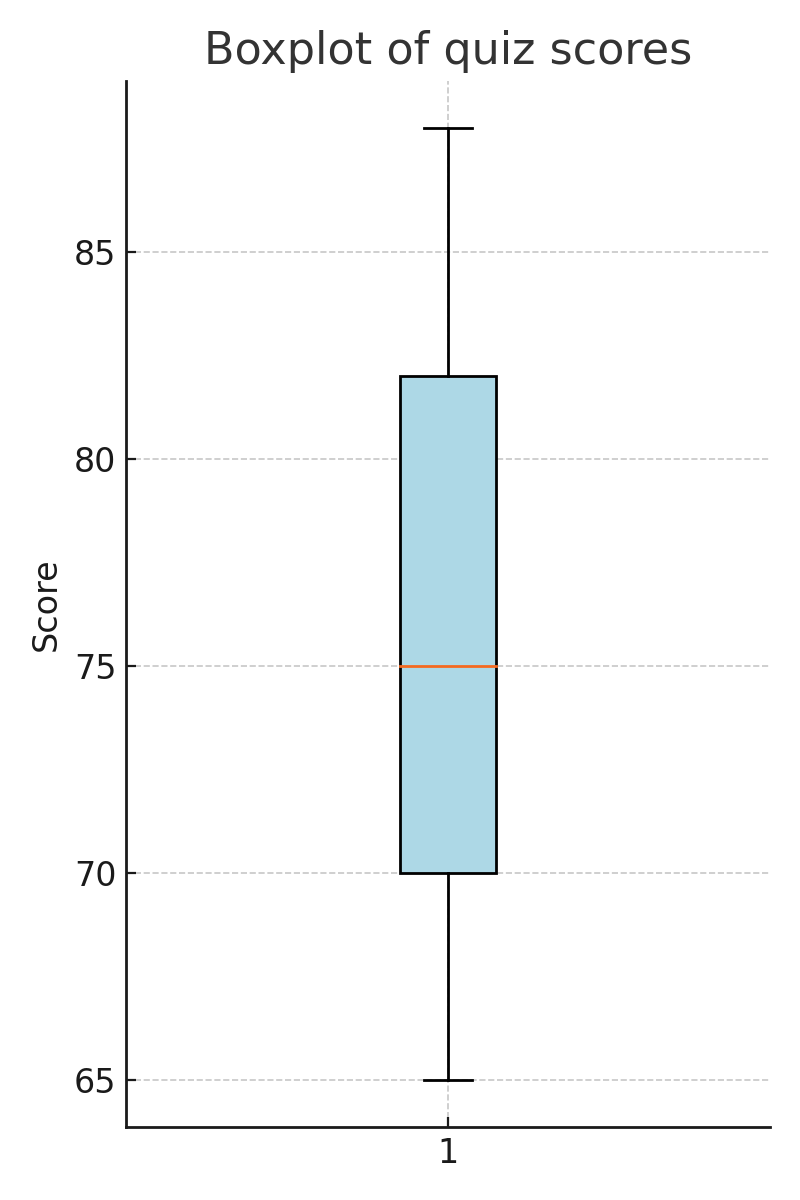
Here’s what the five-number summary from the previous example looks like as a boxplot. Since no values fall outside the $1.5 \times IQR$ fences, the whiskers extend all the way to the actual minimum and maximum.

This example finds an outlier in a data set using the 1.5 IQR rule. It then compares the mean of all values to the mean without the outlier.

Example: identify the outlier and compare means

$10, 12, 15, 14, 13, 100, 16, 14$

Find the following:

The outlier

The mean of all eight values

The mean of the seven typical values excluding the outlier

(spoiler)

Order the data: $10, 12, 13, 14, 14, 15, 16, 100$

First, compute $Q_{1}$ and $Q_{3}$ to find the IQR.

$Q_{1} = \frac{12 + 13}{2} = 12.5$
$Q_{3} = \frac{15 + 16}{2} = 15.5$
$IQR = Q_{3} - Q_{1} = 15.5 - 12.5 = 3$

Now apply the $1.5 \times IQR$ rule. A value is an outlier if it exceeds $Q_{3} + 1.5 \times IQR$ :

Upper outlier bound: $Q_{3} + 1.5 \times IQR = 15.5 + (1.5 \times 3) = 15.5 + 4.5 = 20$

Since $100 > 20$ , it is an outlier.

Mean of all values: $\frac{10 + 12 + 13 + 14 + 14 + 15 + 16 + 100}{8} = \frac{194}{8} = 24.25$
Mean without outlier: $\frac{94}{7} \approx 13.43$

Answer: The outlier is $100$ . The mean of all values is $24.25$ , and the mean without the outlier is approximately $13.43$ .

:::

Justifying conclusions with data

Strong conclusions point to specific numbers, trends, or features in the display, and they avoid claims the data can’t support. When describing a trend, name the direction and support it with at least one specific value - for example, “visits increased by $300$ each month from January ( $1, 200$ ) to March ( $1, 800$ ).”

Correlation is not causation. A trend or association between two variables tells you they move together - it doesn’t tell you that one causes the other. For example, ice cream sales and drowning incidents both rise in the summer, but buying ice cream doesn’t cause drownings - both are driven by hot weather that brings more swimming and more ice cream purchases alike. Describing a trend accurately is fine; claiming a cause-and-effect relationship requires more than a pattern in the data.

Inferences from a random sample

A random sample is a group chosen from a larger population so that every member has the same chance of being picked. Because a random sample tends to resemble the population it came from, the proportion you observe in the sample is a reasonable estimate of the proportion in the whole population. To estimate a count for the population, multiply the sample proportion by the population size.

Example: estimating from a random sample

A factory inspects a random sample of $200$ light bulbs and finds $6$ that are defective. About how many of the day’s $5, 000$ bulbs are defective?

Sample proportion: $\frac{6}{200} = 0.03$

Scale to the population: $0.03 \times 5, 000 = 150$

Answer: about $150$ defective bulbs

The result is an estimate, not an exact count - a different random sample would give a slightly different answer. Larger samples give more reliable estimates, and a sample that isn’t random (for example, asking only the students in the library how many hours they study) can’t be trusted to represent the whole population.

Sidenote

Choosing the right display

Use the right display for your data type - this is a frequently tested skill.

Boxplot - numerical data; best for showing distribution and spotting outliers (e.g., comparing test score spreads across two classes)
Histogram - numerical data; best when the shape of the distribution matters. A symmetric histogram has roughly equal tails on both sides; a right-skewed histogram has a longer tail on the right (a few high values pull the mean up); a left-skewed histogram has a longer tail on the left.
Bar graph - categorical data; compares counts or values across distinct groups (e.g., favorite subject by number of students)
Circle graph (pie chart) - categorical data shown as parts of a whole; each slice’s size represents its percentage of the total
Pictograph - counts shown with repeated symbols; a key gives the value of one symbol, and a partial symbol stands for that fraction of it
Line graph - data that changes over time; connects points to show trends (e.g., monthly rainfall over a year)
Stem-and-leaf plot - numerical data; preserves every actual value while showing the shape of the distribution (the “stem” is the leading digit, the “leaf” is the trailing digit)
Table - exact values for quick lookup or side-by-side comparison across categories
Scatterplot - two numerical variables; reveals relationships or correlations (e.g., hours studied vs. exam score) - covered in depth in the next chapter, Interpreting scatterplots

Example: reading a circle graph

A circle graph shows how $400$ students at a school get to campus: $50%$ walk, $25%$ ride the bus, $20%$ are driven by car, and $5%$ bike. How many students ride the bus?

Answer: $400 \times 0.25 = 100$ students ride the bus.

A pictograph shows counts with repeated symbols. A key gives the value of one symbol, and a partial symbol is that fraction of it: if each ● stands for $10$ books, then ●●◐ is $10 + 10 + 5 = 25$ books. When the key is missing but the total is given, let one symbol stand for $x$ and solve.

Example: reading a pictograph

A pictograph shows the books three classes read. Each ● stands for the same number of books, and each ◐ for half as many. Class A has ●●◐, class B has ●●●, and class C has ●◐. Together they read $105$ books. How many books does each ● stand for?

(spoiler)

Count the symbols: $6$ whole ● and $2$ half ◐, so the total is $6 x + 2 \cdot \frac{x}{2} = 7 x$ .

Solve $7 x = 105$ : $x = 15$ .

Answer: each ● stands for $15$ books

Look for overall patterns, trends, clusters, or cycles before focusing on individual values
Identify any values that stand apart and confirm them as outliers using the $1.5 \times IQR$ rule
Use the five-number summary to describe the spread and center of a data set, and represent it visually with a boxplot
Anchor conclusions in specific numeric changes or clear features from the display
Avoid claims that extend beyond what the data actually show
Estimate a population count from a random sample by multiplying the sample proportion by the population size; the result is an estimate, and larger random samples are more reliable
In a pictograph, each symbol stands for the amount in the key and a partial symbol for that fraction of it; given only the total, let one symbol be $x$ and solve

Next | 2.4 Interpreting scatterplots

Interpreting data

Spotting patterns, trends, and outliers

$Outlier if: x > Q_{3} + 1.5 \times IQR or x < Q_{1} - 1.5 \times IQR$

Values beyond this range are often plotted individually as points or small circles.
When outliers are present, the whiskers extend to the most extreme non-outlier values (the adjacent values inside the fence), not to the actual data minimum or maximum.
Outliers can indicate unusual cases, errors in data collection, or natural variability.

Definitions

Cluster: A concentration of data values within a specific range, indicating a subgroup or phase in the data. Clusters show where values tend to group together and can highlight common behaviors or conditions.
Outlier: A data value that is substantially higher or lower than the rest of the data set.
Trend: A general direction in which data values are moving over time or across categories. Trends can be increasing, decreasing, or constant, and they help reveal long-term patterns in a data set.

Finding the five-number summary

We order the data, then find the median. We split the data into a lower half and an upper half to find the first and third quartiles. This gives the five-number summary for the data set.

Take the following data set:

$65, 68, 71, 74, 77, 82, 82, 89$

There are $n = 8$ values, already ordered. The median is the average of the $4^{th}$ and $5^{th}$ values:

$Q_{2} = \frac{74 + 77}{2} = 75.5$

The lower half is $65, 68, 71, 74$ , so:

$Q_{1} = \frac{68 + 71}{2} = 69.5$

The upper half is $77, 82, 82, 89$ , so:

$Q_{3} = \frac{82 + 82}{2} = 82$

This gives the five-number summary:

Minimum (Min) = $65$
First quartile ( $Q_{1}$ ) = $69.5$
Median ( $Q_{2}$ ) = $75.5$
Third quartile ( $Q_{3}$ ) = $82$
Maximum (Max) = $89$

Sidenote

Watch out

Always order the data before computing any quartile. A common mistake is reading $Q_{1}$ as the smallest value in the lower half - it’s actually the median of the lower half.

Visual interpretation

This example finds an outlier in a data set using the 1.5 IQR rule. It then compares the mean of all values to the mean without the outlier.

Example: identify the outlier and compare means

$10, 12, 15, 14, 13, 100, 16, 14$

Find the following:

The outlier

The mean of all eight values

The mean of the seven typical values excluding the outlier

(spoiler)

Order the data: $10, 12, 13, 14, 14, 15, 16, 100$

First, compute $Q_{1}$ and $Q_{3}$ to find the IQR.

$Q_{1} = \frac{12 + 13}{2} = 12.5$
$Q_{3} = \frac{15 + 16}{2} = 15.5$
$IQR = Q_{3} - Q_{1} = 15.5 - 12.5 = 3$

Now apply the $1.5 \times IQR$ rule. A value is an outlier if it exceeds $Q_{3} + 1.5 \times IQR$ :

Upper outlier bound: $Q_{3} + 1.5 \times IQR = 15.5 + (1.5 \times 3) = 15.5 + 4.5 = 20$

Since $100 > 20$ , it is an outlier.

Mean of all values: $\frac{10 + 12 + 13 + 14 + 14 + 15 + 16 + 100}{8} = \frac{194}{8} = 24.25$
Mean without outlier: $\frac{94}{7} \approx 13.43$

Answer: The outlier is $100$ . The mean of all values is $24.25$ , and the mean without the outlier is approximately $13.43$ .

:::

Justifying conclusions with data

Inferences from a random sample

Example: estimating from a random sample

A factory inspects a random sample of $200$ light bulbs and finds $6$ that are defective. About how many of the day’s $5, 000$ bulbs are defective?

Sample proportion: $\frac{6}{200} = 0.03$

Scale to the population: $0.03 \times 5, 000 = 150$

Answer: about $150$ defective bulbs

Sidenote

Choosing the right display

Use the right display for your data type - this is a frequently tested skill.

Boxplot - numerical data; best for showing distribution and spotting outliers (e.g., comparing test score spreads across two classes)
Histogram - numerical data; best when the shape of the distribution matters. A symmetric histogram has roughly equal tails on both sides; a right-skewed histogram has a longer tail on the right (a few high values pull the mean up); a left-skewed histogram has a longer tail on the left.
Bar graph - categorical data; compares counts or values across distinct groups (e.g., favorite subject by number of students)
Circle graph (pie chart) - categorical data shown as parts of a whole; each slice’s size represents its percentage of the total
Pictograph - counts shown with repeated symbols; a key gives the value of one symbol, and a partial symbol stands for that fraction of it
Line graph - data that changes over time; connects points to show trends (e.g., monthly rainfall over a year)
Stem-and-leaf plot - numerical data; preserves every actual value while showing the shape of the distribution (the “stem” is the leading digit, the “leaf” is the trailing digit)
Table - exact values for quick lookup or side-by-side comparison across categories
Scatterplot - two numerical variables; reveals relationships or correlations (e.g., hours studied vs. exam score) - covered in depth in the next chapter, Interpreting scatterplots

Example: reading a circle graph

A circle graph shows how $400$ students at a school get to campus: $50%$ walk, $25%$ ride the bus, $20%$ are driven by car, and $5%$ bike. How many students ride the bus?

Answer: $400 \times 0.25 = 100$ students ride the bus.

Example: reading a pictograph

A pictograph shows the books three classes read. Each ● stands for the same number of books, and each ◐ for half as many. Class A has ●●◐, class B has ●●●, and class C has ●◐. Together they read $105$ books. How many books does each ● stand for?

(spoiler)

Count the symbols: $6$ whole ● and $2$ half ◐, so the total is $6 x + 2 \cdot \frac{x}{2} = 7 x$ .

Solve $7 x = 105$ : $x = 15$ .

Answer: each ● stands for $15$ books

Achievable Praxis Core: Math (5733)

2. Data analysis, statistics, and probability