



Inventory systems: perpetual
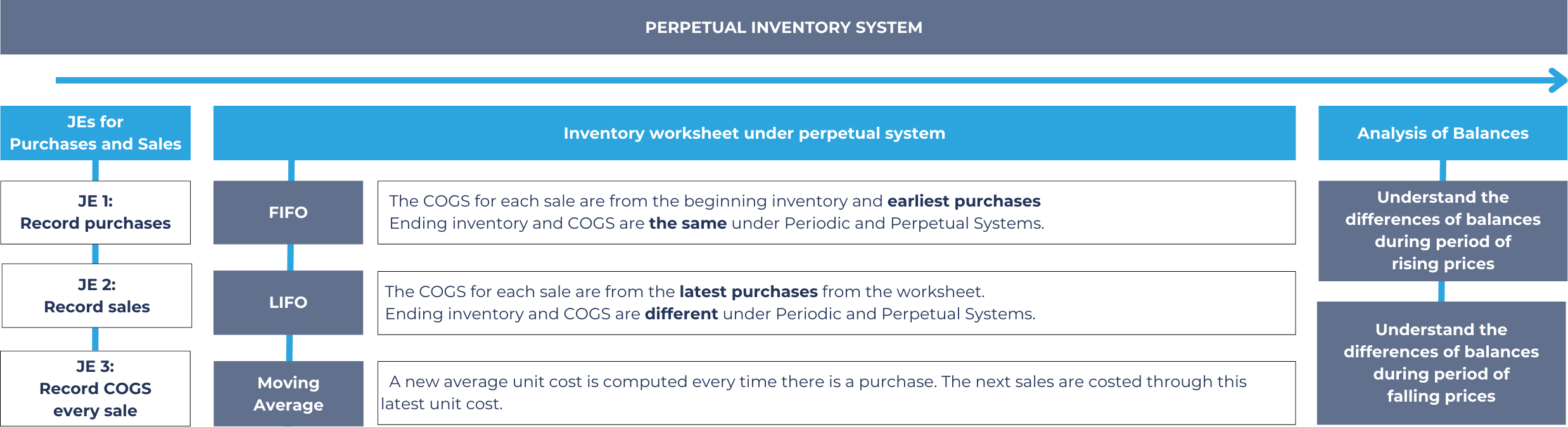
The following concept map for the perpetual inventory system could be helpful to navigate through the topic:
Perpetual inventory system
The perpetual inventory system is the opposite of the periodic inventory system in a way that the inventory is updated in real time as purchases and sales happen, and the cost of goods sold is determined every sale, instead of both being determined at the end of the period.
However, despite this difference, the different cost flow assumptions are still used in the analyses.
Journal entries under the perpetual system
Under the perpetual inventory system, a journal entry is generated at each purchase and sale that shows the effects of the transactions to the company’s inventory and cost of goods sold immediately. This is the main difference of this system versus the periodic inventory system, which determines these balances through the year-end procedures only.
Since each purchase/sale transaction generates a separate journal entry, in practice these will be numerous but repetitive in nature, hence we will only show the pro forma journal entries in this section to familiarize you with them. All these entries will be applicable to each transaction that will be shown in the worksheets of the succeeding sections.
The journal entry to record a purchase increases the “inventory” account on the balance sheet instead of a “purchases” account on the income statement. There are then two journal entries every time a sale occurs: one for the sale itself (the same entry used under the periodic system), and one for the cost of goods sold (only recorded under the perpetual system). The second entry reduces the inventory balance and transfers that cost to COGS with each sale.
| Entry | Account | Debit | Credit | Financial statement element |
|---|---|---|---|---|
| JE 1 - record purchase | Inventory | XXX | Asset | |
| Cash or accounts payable | XXX | Asset or liability | ||
| JE 2 - record sale | Cash or accounts receivable | XXX | Asset | |
| Sales revenue | XXX | Revenue | ||
| JE 3 - record COGS | Cost of goods sold | XXX | Expense | |
| Inventory | XXX | Asset |
There will be no year-end procedures and adjustments under the perpetual inventory system because the inventory and COGS accounts in the balance sheet and income statement, respectively, are being updated by the journal entries in real-time.
Inventory worksheet under perpetual system
Unlike the periodic inventory system, which is easily learned using journal entries, the perpetual inventory system is best learned using inventory worksheets, prepared slightly differently for each cost flow assumption.
From here, we can analyze the impacts of each transaction instead of just the ending balances. We will use the same facts in the exercise used in the periodic inventory system to be able to compare the results with the perpetual inventory system.
FIFO perpetual assumption
Before working through a perpetual worksheet, you should know that FIFO periodic and FIFO perpetual always produce the same ending inventory and COGS balances - $7,500 and $5,000 in this example. That’s because FIFO always assigns the earliest purchases to COGS first, regardless of when each sale happens during the period, so the order in which you match units to costs doesn’t change the outcome. If you’re asked to compute FIFO perpetual, you can use the faster FIFO periodic method (shown in the previous chapter) and arrive at the same result.
LIFO perpetual assumption
Under the LIFO perpetual assumption, the ending inventory of 2,000 units can only be determined using an inventory worksheet because LIFO periodic and LIFO perpetual results in different inventory and COGS balances at the end of the period.
| Date | Nature | Transactions | Inventory | Cost of goods sold | ||||||
| Units | Cost | Total | Units | Cost | Total | Units | Cost | Total | ||
| Apr 1 | Beginning inventory | 500 | $2.0 | $1,000 | 500 | $2.0 | $1,000 | |||
| Apr 2 | Purchase | 1,000 | $2.5 | $2,500 | 1,000 | $2.5 | $2,500 | |||
| Apr 5 | Purchase | 1,000 | $3.0 | $3,000 | 1,000 | $3.0 | $3,000 | |||
| Apr 9 | Sale (Per unit: $7.00) | (800) | ||||||||
| From Apr 5 purchase | (800) | $3.0 | ($2,400) | 800 | $3.0 | $2,400 | ||||
| Apr 15 | Purchase | 1,500 | $4.0 | $6,000 | 1,500 | $4.0 | $6,000 | |||
| Apr 29 | Sale (Per unit: $8.00) | (1,200) | ||||||||
| From Apr 15 purchase | (1,200) | $4.0 | ($4,800) | 1,200 | $4.0 | $4,800 | ||||
| Apr 30 | Ending inventory | 2,000 | $12,500 | 2,000 | $5,300 | 2,000 | $7,200 | |||
The difference with FIFO perpetual is that the sales are attributed to the latest inventories purchased.
You will notice that the total inventories ($ 5,300) and the COGS ($ 7,200) are still equal to the cost of goods available for sale of $ 12,500. This will be true for all methods and cost flow assumptions we will discuss.
Moving average assumption
Under the perpetual inventory system, the average method is called the moving average method because for every purchase, the average inventory cost is computed and there is no single average cost of inventory unlike the weighted average method in the periodic inventory system.
| Date | Nature | Transactions | Inventory | Cost of goods sold | ||||||
| Units | Cost | Total | Units | Avg. cost | Total | Units | Avg. cost | Total | ||
| Apr 1 | Beginning inventory | 500 | $2.0 | $1,000 | 500 | $2.0 | $1,000 | |||
| Apr 2 | Purchase | 1,000 | $2.5 | $2,500 | 1,000 | $2.5 | $2,500 | |||
| Apr 5 | Purchase | 1,000 | $3.0 | $3,000 | 1,000 | $3.0 | $3,000 | |||
| Average cost/ accumulated balance | 2,500 | $2.6 | $6,500 | |||||||
| Apr 9 | Sale (Per unit: $7.00) | (800) | (800) | $2.6 | ($2,080) | 800 | $2.6 | $2,080 | ||
| Apr 15 | Purchase | 1,500 | $4.0 | $6,000 | 1,500 | $4.0 | $6,000 | |||
| Average cost/ accumulated balance | 3,200 | $3.26 | $10,420 | |||||||
| Apr 29 | Sale (Per unit: $8.00) | (1,200) | (1,200) | $3.26 | ($3,912) | 1,200 | $3.26 | $3,912 | ||
| Apr 30 | Ending inventory | 2,000 | $12,500 | 2,000 | $6,508 | 2,000 | $5,992 | |||
You need to compute the average cost of inventory after every purchase. In this case we have skipped the first two purchases as it would have no impact since the first sale happened on April 9.
Analysis of the ending balances under the perpetual system
Below is a summary of the ending inventory, sales, cost of goods sold and gross profit under all cost flow assumptions of the perpetual inventory system. Good thing to remember is that April is a period of rising prices for the company.
| Units | FIFO | LIFO | Moving ave. | |
| Balance sheet: | ||||
| Ending inventory | 2,000 | $ 7,500 | $ 5,300 | $ 6,508 |
| Income statement: | ||||
| Sales* | 2,000 | $ 15,200 | $ 15,200 | $ 15,200 |
| Cost of goods sold | 2,000 | ($ 5,000) | ($ 7,200) | ($ 5,992) |
| Gross profit | $ 10,200 | $ 8,000 | $ 9,208 |
The amount of sales is the total sales (Apr 9 and Apr 29) from the example.
In a period of rising prices, the following are proven from the exercise:
- FIFO method has the highest gross profit because the cost of goods sold are based on the lower priced inventory items of the old purchases
- In effect of above, in a period of rising prices, LIFO has a higher cost of goods sold
- FIFO has the higher cost of ending inventory in the balance sheet because these are based on the higher priced most current purchases
- The average method is expected to be in the middle of both FIFO and LIFO.
Also we observed the following when comparing the different methods and systems:
- FIFO perpetual and FIFO periodic result in the same amounts of ending inventory and COGS
- LIFO perpetual does not always result in the same balances as LIFO periodic
- The moving average method does not result in the same balances as the weighted average method