2.3.2.2 Learning curve calculation

Achievable CMA Part 1

2. Planning, budgeting, and forecasting

2.3. Forecasting techniques

2.3.2. Learning curve analysis

Our CMA Part 1 course is currently in development and is a work-in-progress.

Learning curve calculation

8 min read

Font

Discuss

Feedback

Calculating the learning curve

The cumulative average-time learning model is one of the most commonly used models in learning curve analysis. It calculates the average time or cost per unit based on the cumulative number of units produced.

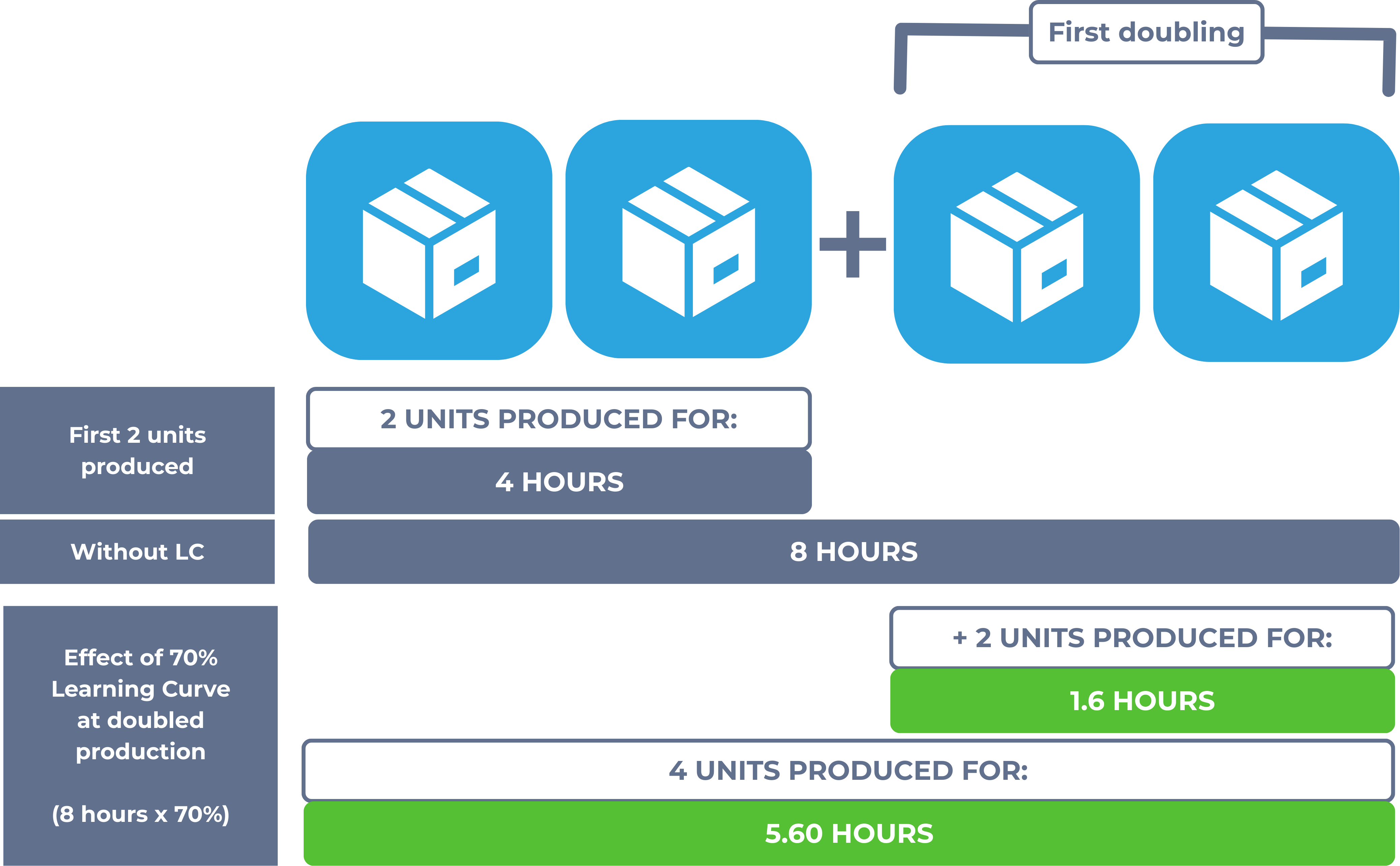
In a learning curve, the production time decreases as cumulative production increases. For instance, if a company operates with a 70% learning curve, each time the total number of units produced doubles, the cumulative production time for all units drops to 70% of what it would have been if there were no learning effect. In the absence of learning, doubling production would simply double the time required.

The cumulative average-time learning model can be applied to calculate the following metrics:

Total production time or cost: This is the total time (or cost) required to produce the entire quantity of units, from the first unit to the last. It takes into account the efficiency improvements gained as production increases.
Cumulative average time per unit: This refers to the average time taken to produce each unit, calculated from the very first unit produced to the final unit in the total quantity. This average reflects the efficiency gained across all units due to the learning process.

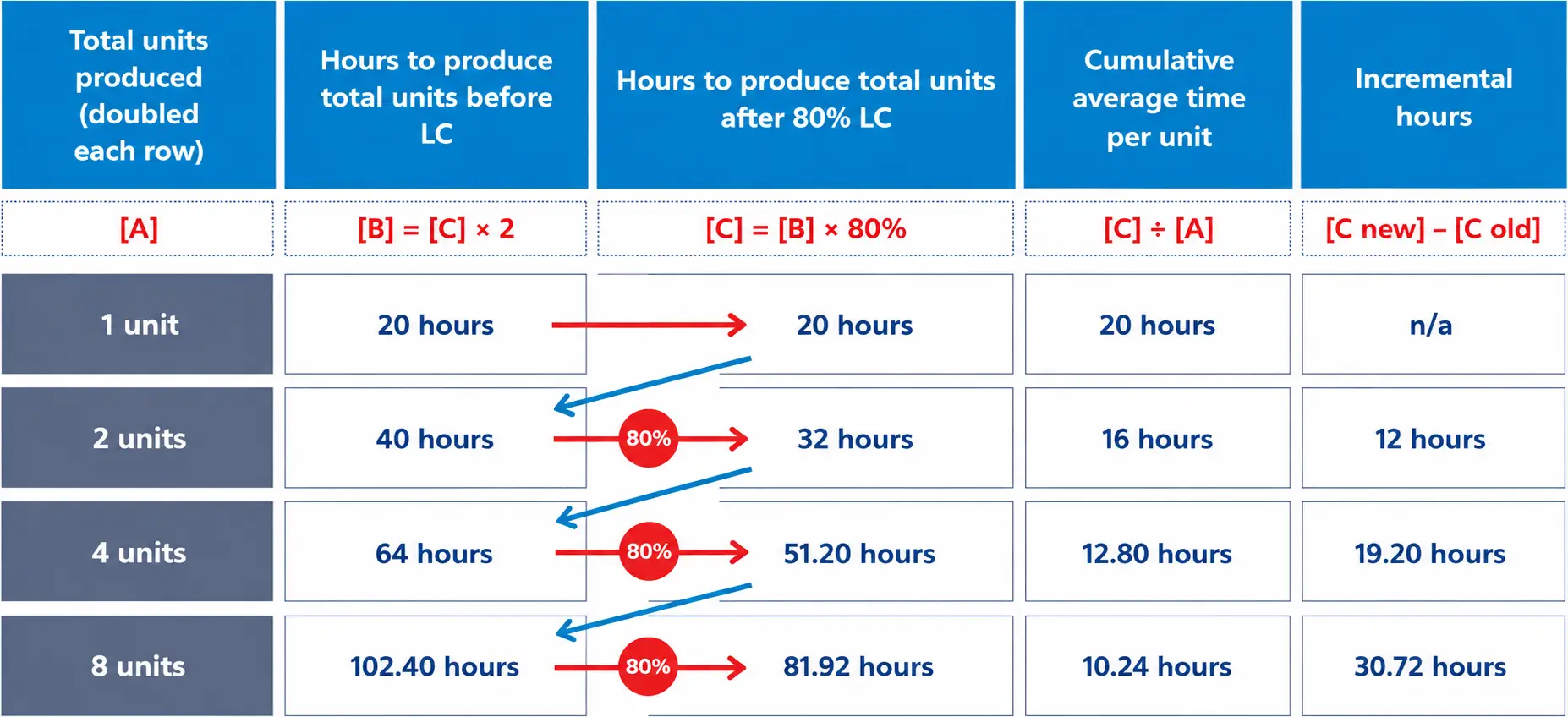
Example: See the following summary of production capacities for a company that manufactures model cars. The first unit takes $20 hours$ to produce and the company has determined that an $80% learning curve$ is applicable.

Calculating cumulative average and incremental hours for units produced under an 80% learning curve. — Learning Curve Example

In terms of the total production time and incremental time, the following interpretations can be inferred from the table:

If the company produces only one unit, it will take 20 hours.
Producing the second unit (the first doubling of production) will take a total of 32 hours, or an additional 12 hours from the original 20 hours it took to produce the first car. As a result, instead of 20 hours, it will only take 12 hours to produce the 2nd car.
Producing a total of 4 units (the second doubling of the production) will take only a total of 51.2 hours, or an additional 19.2 hours from the first 2 that was produced. As a result, 19.2 hours would be the hours required to produce the 3rd and 4th cars.
Producing a total of 8 units (the third doubling of the production) will take a total of 81.92 hours, or an additional 30.72 hours from the first 4 that was produced. As a result, it will take 30.72 hours to produce the 5th to 8th cars.

In terms of the cumulative average time per unit, you will notice that the average time decreased as the production is doubled. By the time the 8th car is produced, it only takes an average of 10.24 hours to produce the last unit, compared to 20 hours required to produce the first.

All the calculations above can be represented in the following formula:

$Y = (a)(2LC)^{n}$

Where:

Y = Total production time to produce all units
a = the time or cost to produce the first unit
LC = the learning curve in decimals
n = the number of doublings to date

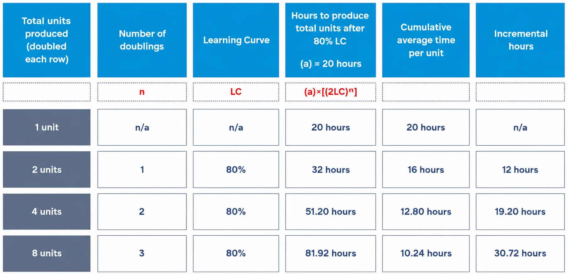
Applying the above formula to the same example we have the following table below. Note that $a = 20 hours$ , which is the number of hours to produce the first car.

Applying the learning curve formula to calculate hours per unit as production doubles. — Learning Curve Formula

Notice that it will produce the same results as the previous solution.

The learning curve analysis can manifest in different ways in the exam but the key is understanding the concepts behind it. CMA candidates can be asked about:

the total production time
the average time per unit; or
the incremental time required to produce additional batches.

Let’s take the following example problem:

Example 1: EcoDrive Technologies is launching a new line of electric motors for eco-friendly vehicles. As the production team gains experience, EcoDrive expects a reduction in production time due to improved efficiency. Based on past experience, the company projects a 80% learning curve. The cost to produce the first motor is estimated at $10,000.

Required: What is the estimated cost of manufacturing an additional seven (7) motors after the first one has been completed (8 total units)?

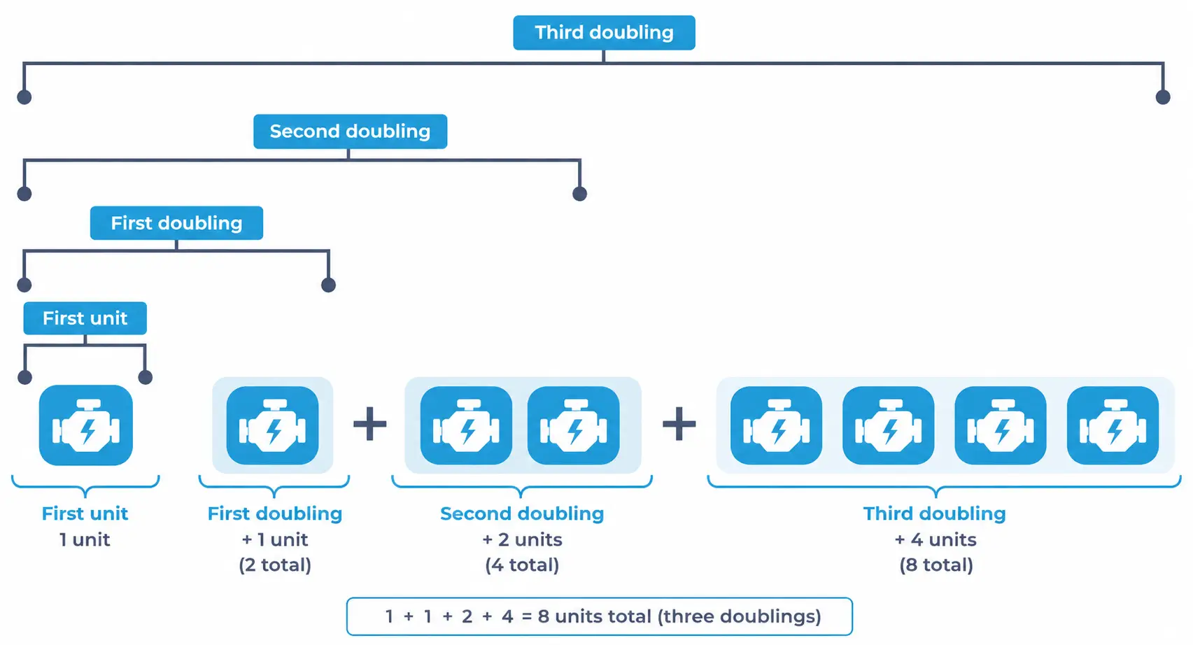
Solution: Manufacturing an additional seven (7) motors mean that production has already doubled thrice from the original one that was produced.

Showing successive doublings of production from one unit through the third doubling. — Doubling of Production

Using the formula:

$Y = (a)(2LC)^{n}$

where:

$Y$ is the total cost of producing 8 units,
$n = 3$ which the number of doublings at the production level of 8 units
$a = $10, 000$ which is the cost of producing the original batch; and
$LC = 80%$ which is EcoDrive’s learning curve,

we can compute the total cost of producing 8 units.

$Cost to manufacture 8 units = (a)(2LC)^{n} = ($10, 000) (2 \times 80%)^{3} = ($10, 000) (1.60)^{3} = ($10, 000) (4.096) = $40, 960$

This means that if the first unit costs $10,000 to produce, then the cost of the next seven units will be:

$Cost of the next seven (7) units = $40, 960 - $10, 000 = $30, 960$

CMA candidates can also be asked to do a simple estimation of the learning curve percentage like as follows:

Example 2: Nova Robotics took 10,000 hours to produce its first batch of 100 units. When production doubled to 200 units, the total labor time amounted to 16,000 hours.

Required: What is the learning curve percentage of Nova Robotics?

Explanation: The hours without efficiency would have been: $2 \times 10, 000 hours = 20, 000 hours$ .

To calculate the learning curve, divide the time for 200 units (after the efficiency gains) by the time for 200 units (without the efficiency gains): $16, 000 hours /20, 000 hours = 80%$ .

Conclusion

Learning curve analysis is an essential tool for forecasting labor efficiency improvements and cost reductions over time, especially in industries with repetitive processes. By using models such as the cumulative average-time learning model, businesses can predict how production time or costs will decrease as workers gain experience. This technique is highly useful in budgeting and planning, as it allows organizations to project labor costs, allocate resources efficiently, and optimize pricing strategies based on anticipated efficiency gains.

However, it is important to recognize the limitations of the learning curve percentage used in these models. The learning curve should ideally be above 50% and below 100%. A percentage below 50% would indicate unrealistically high efficiency gains, while a percentage of 100% or higher suggests no improvement at all. Businesses typically use learning curves between 70% and 90% to reflect realistic improvements based on industry and process complexity.

In practice, learning curve analysis provides valuable insights, but it must be applied carefully, considering factors like process stability, data accuracy, and the inherent limits to human and machine efficiency. When applied correctly, it can enhance an organization’s ability to plan production, control costs, and remain competitive in dynamic markets.

Cumulative Average-Time Learning Model

Calculates average time/cost per unit based on cumulative units produced
Each time cumulative production doubles, total production time drops to the learning curve % of what it would be without learning

Learning Curve Formula

$Y = (a)(2LC)^{n}$
$Y$ = total production time/cost, $a$ = time/cost for first unit, $LC$ = learning curve (decimal), $n$ = number of doublings
Incremental time for additional batches = total time at new level minus total time at prior level

Key Metrics on Exams

Three common question types: total production time, average time per unit, or incremental time for additional batches
Learning curve % can be derived: divide actual total time after doubling by expected time without efficiency gains

Limitations and Valid Range

Learning curve should be between 50% and 100%
- Below 50%: unrealistically high efficiency gains
- At or above 100%: implies no improvement
Typical industry range: 70%–90%

Applications

Used in budgeting, labor cost projection, resource allocation, and pricing strategy
Most relevant for repetitive processes where worker experience drives efficiency gains

Next | 2.3.3 Expected value

Learning curve calculation

Calculating the learning curve

The cumulative average-time learning model can be applied to calculate the following metrics:

Total production time or cost: This is the total time (or cost) required to produce the entire quantity of units, from the first unit to the last. It takes into account the efficiency improvements gained as production increases.
Cumulative average time per unit: This refers to the average time taken to produce each unit, calculated from the very first unit produced to the final unit in the total quantity. This average reflects the efficiency gained across all units due to the learning process.

In terms of the total production time and incremental time, the following interpretations can be inferred from the table:

If the company produces only one unit, it will take 20 hours.
Producing the second unit (the first doubling of production) will take a total of 32 hours, or an additional 12 hours from the original 20 hours it took to produce the first car. As a result, instead of 20 hours, it will only take 12 hours to produce the 2nd car.
Producing a total of 4 units (the second doubling of the production) will take only a total of 51.2 hours, or an additional 19.2 hours from the first 2 that was produced. As a result, 19.2 hours would be the hours required to produce the 3rd and 4th cars.
Producing a total of 8 units (the third doubling of the production) will take a total of 81.92 hours, or an additional 30.72 hours from the first 4 that was produced. As a result, it will take 30.72 hours to produce the 5th to 8th cars.

All the calculations above can be represented in the following formula:

$Y = (a)(2LC)^{n}$

Where:

Y = Total production time to produce all units
a = the time or cost to produce the first unit
LC = the learning curve in decimals
n = the number of doublings to date

Applying the above formula to the same example we have the following table below. Note that $a = 20 hours$ , which is the number of hours to produce the first car.

Notice that it will produce the same results as the previous solution.

The learning curve analysis can manifest in different ways in the exam but the key is understanding the concepts behind it. CMA candidates can be asked about:

the total production time
the average time per unit; or
the incremental time required to produce additional batches.

Let’s take the following example problem:

Required: What is the estimated cost of manufacturing an additional seven (7) motors after the first one has been completed (8 total units)?

Solution: Manufacturing an additional seven (7) motors mean that production has already doubled thrice from the original one that was produced.

Using the formula:

$Y = (a)(2LC)^{n}$

where:

$Y$ is the total cost of producing 8 units,
$n = 3$ which the number of doublings at the production level of 8 units
$a = $10, 000$ which is the cost of producing the original batch; and
$LC = 80%$ which is EcoDrive’s learning curve,